使用python基于Streamlit构建的跨城市人类移动行为预测系统,利用迁移学习技术将源城市的丰富数据知识迁移到目标城市进行流量预测。
一、整体设计
1. 应用类型
-
交互式Web应用:使用Streamlit构建,支持实时数据生成、模型训练、预测和可视化
-
数据科学演示系统:展示迁移学习在时空预测中的应用
2. 技术栈分层
-
前端展示层:Streamlit + Plotly + Matplotlib/Seaborn
-
模型算法层:Scikit-learn RandomForest + 自定义迁移学习逻辑
-
数据处理层:Pandas + NumPy
-
可视化层:多图表联动展示
二、核心功能模块
1. 数据生成模块 (generate_city_data)
创新点:
-
模拟不同城市的交通流量特征
-
北京:早晚高峰明显(典型上班族模式)
-
上海:夜间经济活跃(商业城市特征)
-
深圳:夜间活动较少(制造业城市特征)
技术细节:
# 时空特征构建
hour_pattern = [0.3, 0.2, 0.1, ...]  # 24小时模式
weekday_factor = np.where(dates.weekday < 5, 1.0, 0.8)  # 工作日/周末差异
region_factor = np.random.uniform(0.7, 1.3)  # 区域异质性
2. 可视化引擎
桑基图分析 (prepare_sankey_data):
-
将一天分为4个时段:深夜、上午、下午、晚上
-
展示区域-时段流量分布关系
-
连线宽度表示流量强度,直观展示时空模式
多维度图表:
-
时间序列图:区域流量随时间变化
-
桑基图:区域流量时空分布
-
热力图:区域×小时流量矩阵
-
对比图:跨城市模式对比
-
预测图:历史+未来预测
-
误差分析图:预测vs实际散点
3. 迁移学习模型 (CrossCityTransferModel)
特征工程创新
# 周期性特征(处理时间序列的周期性)
hour_sin = sin(2π * hour / 24)  # 保持周期性
hour_cos = cos(2π * hour / 24)

# 滞后特征(捕捉时间依赖性)
df['traffic_lag_1']  # 1小时前
df['traffic_lag_24']  # 24小时前(日周期)

# 滚动统计特征
df['traffic_rolling_mean_6']  # 6小时移动平均
df['traffic_rolling_std_12']   # 12小时移动标准差
迁移策略
-
源域训练:在数据丰富的源城市训练完整模型
-
目标域适配:
-
直接迁移:直接应用源模型
-
微调迁移:用少量目标数据微调模型参数
-
-
特征对齐:确保源域和目标域特征空间一致
4. 预测模块
创新性:多步滚动预测
# 自回归预测
for hour in range(hours_ahead):
    # 1. 更新未来时间点的时间特征
    # 2. 用最新预测值更新滞后特征
    # 3. 预测下一个时间点
    # 4. 将预测值加入历史序列
三、工作流程
阶段1:数据生成与探索
用户选择城市 → 生成模拟数据 → 可视化探索 → 理解数据模式阶段2:模型训练与迁移
源城市训练 → 特征提取 → 迁移到目标城市 → 评估性能阶段3:预测与分析
选择区域 → 生成预测 → 结果可视化 → 下载预测结果四、完整代码
import streamlit as st
import pandas as pd
import numpy as np
import plotly.graph_objects as go
import plotly.express as px
from plotly.subplots import make_subplots
import matplotlib.pyplot as plt
import seaborn as sns
from datetime import datetime, timedelta
import random
from sklearn.ensemble import RandomForestRegressor
from sklearn.preprocessing import StandardScaler
from sklearn.model_selection import train_test_split
from sklearn.metrics import mean_absolute_error, mean_squared_error, r2_score
import warnings
warnings.filterwarnings('ignore')
# 设置页面配置
st.set_page_config(
page_title="跨城市人类移动行为",
page_icon="🏙️",
layout="wide"
)
# 应用标题和描述
st.title("跨城市人类移动行为")
st.markdown("""
基于迁移学习的跨城市流量预测,通过源城市的丰富数据预测目标城市的移动模式。
""")
# 侧边栏
st.sidebar.header("系统配置")
# 模拟数据生成函数
@st.cache_data
def generate_city_data(city_name, n_days=30, n_regions=20, seed=42):
"""生成城市移动数据"""
np.random.seed(seed)
# 生成日期范围
dates = pd.date_range(start='2024-01-01', periods=n_days * 24, freq='H')
# 为不同城市设置不同的流量模式
if city_name == "北京":
base_traffic = np.random.normal(1000, 200, len(dates))
# 北京的早晚高峰更明显
hour_pattern = np.array([0.3, 0.2, 0.1, 0.1, 0.2, 0.5, 1.2, 1.8, 1.5, 1.2, 1.1, 1.0,
1.0, 0.9, 1.0, 1.2, 1.5, 1.8, 1.6, 1.3, 1.0, 0.7, 0.5, 0.4])
elif city_name == "上海":
base_traffic = np.random.normal(900, 180, len(dates))
# 上海的夜间经济更活跃
hour_pattern = np.array([0.4, 0.3, 0.2, 0.2, 0.3, 0.6, 1.0, 1.5, 1.4, 1.3, 1.2, 1.1,
1.1, 1.0, 1.1, 1.3, 1.6, 1.7, 1.8, 1.6, 1.3, 1.0, 0.7, 0.5])
elif city_name == "深圳":
base_traffic = np.random.normal(800, 150, len(dates))
# 深圳的夜间活动较少
hour_pattern = np.array([0.2, 0.1, 0.1, 0.1, 0.2, 0.4, 1.0, 1.6, 1.5, 1.3, 1.2, 1.1,
1.1, 1.0, 1.1, 1.2, 1.4, 1.5, 1.3, 1.1, 0.9, 0.6, 0.4, 0.3])
else: # 目标城市
base_traffic = np.random.normal(700, 120, len(dates))
hour_pattern = np.array([0.3, 0.2, 0.1, 0.1, 0.2, 0.5, 1.1, 1.6, 1.4, 1.2, 1.1, 1.0,
1.0, 0.9, 1.0, 1.1, 1.3, 1.4, 1.3, 1.1, 0.9, 0.6, 0.4, 0.3])
# 应用小时模式
hour_indices = dates.hour.values
hour_factors = hour_pattern[hour_indices]
# 生成区域数据
data = []
for region_id in range(n_regions):
# 为每个区域添加一些独特性
region_factor = np.random.uniform(0.7, 1.3)
# 工作日/周末模式
weekday_factor = np.where(dates.weekday < 5, 1.0, 0.8)
# 生成流量
region_traffic = base_traffic * hour_factors * weekday_factor * region_factor
region_traffic = np.maximum(region_traffic, 0) # 确保非负
# 添加一些随机噪声
noise = np.random.normal(0, 50, len(region_traffic))
region_traffic += noise
for i, date in enumerate(dates):
data.append({
'datetime': date,
'region_id': region_id,
'city': city_name,
'traffic_volume': int(region_traffic[i]),
'hour': date.hour,
'day_of_week': date.weekday(),
'is_weekend': 1 if date.weekday() >= 5 else 0,
'month': date.month,
'day': date.day
})
df = pd.DataFrame(data)
return df
# 生成桑基图数据的函数
def prepare_sankey_data(city_data, top_n_regions=5):
"""准备桑基图数据,展示区域间的流量关系"""
if city_data is None or len(city_data) == 0:
return None, None, None
# 选择流量最高的前N个区域
region_totals = city_data.groupby('region_id')['traffic_volume'].sum().sort_values(ascending=False)
top_regions = region_totals.head(top_n_regions).index.tolist()
# 筛选出前N个区域的数据
top_data = city_data[city_data['region_id'].isin(top_regions)].copy()
# 将一天分为4个时段
def get_time_period(hour):
if 0 <= hour < 6:
return '深夜 (0-6点)'
elif 6 <= hour < 12:
return '上午 (6-12点)'
elif 12 <= hour < 18:
return '下午 (12-18点)'
else:
return '晚上 (18-24点)'
top_data['time_period'] = top_data['hour'].apply(get_time_period)
# 计算每个区域在每个时段的平均流量
period_flow = top_data.groupby(['region_id', 'time_period'])['traffic_volume'].mean().reset_index()
# 为桑基图准备节点
regions = [f'区域 {int(r)}' for r in top_regions]
time_periods = ['深夜 (0-6点)', '上午 (6-12点)', '下午 (12-18点)', '晚上 (18-24点)']
# 所有节点
nodes = regions + time_periods
# 创建源节点、目标节点和流量值
source = []
target = []
value = []
# 区域节点索引
region_indices = {f'区域 {int(r)}': i for i, r in enumerate(top_regions)}
# 时段节点索引(在区域节点之后)
time_indices = {tp: len(regions) + i for i, tp in enumerate(time_periods)}
for _, row in period_flow.iterrows():
region_label = f'区域 {int(row["region_id"])}'
time_label = row['time_period']
flow_value = row['traffic_volume']
source.append(region_indices[region_label])
target.append(time_indices[time_label])
value.append(flow_value)
return nodes, source, target, value, period_flow
# 迁移学习模型
class CrossCityTransferModel:
def __init__(self):
self.source_model = RandomForestRegressor(n_estimators=100, random_state=42)
self.target_model = RandomForestRegressor(n_estimators=50, random_state=42)
self.scaler = StandardScaler()
self.is_fitted = False
def create_features(self, df):
"""创建特征"""
df_features = df.copy()
# 时间特征
df_features['hour_sin'] = np.sin(2 * np.pi * df_features['hour'] / 24)
df_features['hour_cos'] = np.cos(2 * np.pi * df_features['hour'] / 24)
df_features['day_sin'] = np.sin(2 * np.pi * df_features['day_of_week'] / 7)
df_features['day_cos'] = np.cos(2 * np.pi * df_features['day_of_week'] / 7)
# 滞后特征
for lag in [1, 2, 3, 24]:
df_features[f'traffic_lag_{lag}'] = df.groupby('region_id')['traffic_volume'].shift(lag)
# 滚动统计特征
for window in [3, 6, 12]:
df_features[f'traffic_rolling_mean_{window}'] = df.groupby('region_id')['traffic_volume'].transform(
lambda x: x.rolling(window, min_periods=1).mean())
df_features[f'traffic_rolling_std_{window}'] = df.groupby('region_id')['traffic_volume'].transform(
lambda x: x.rolling(window, min_periods=1).std())
# 区域特征
region_stats = df.groupby('region_id')['traffic_volume'].agg(['mean', 'std', 'max']).reset_index()
region_stats.columns = ['region_id', 'region_mean', 'region_std', 'region_max']
df_features = pd.merge(df_features, region_stats, on='region_id', how='left')
# 删除缺失值
df_features = df_features.dropna()
return df_features
def train_on_source(self, source_df):
"""在源城市数据上训练"""
st.info(f"正在使用源城市数据训练模型,数据量: {len(source_df):,} 条记录")
# 创建特征
source_features = self.create_features(source_df)
# 准备特征和目标变量
feature_cols = [col for col in source_features.columns if col not in
['traffic_volume', 'datetime', 'city', 'region_id', 'hour', 'day_of_week', 'month', 'day']]
X = source_features[feature_cols]
y = source_features['traffic_volume']
# 标准化特征
X_scaled = self.scaler.fit_transform(X)
# 训练模型
self.source_model.fit(X_scaled, y)
# 评估模型
y_pred = self.source_model.predict(X_scaled)
mae = mean_absolute_error(y, y_pred)
rmse = np.sqrt(mean_squared_error(y, y_pred))
r2 = r2_score(y, y_pred)
st.success(f"源城市模型训练完成 - MAE: {mae:.1f}, RMSE: {rmse:.1f}, R²: {r2:.3f}")
return feature_cols, mae, rmse, r2
def transfer_to_target(self, target_df, feature_cols, fine_tune=True):
"""迁移到目标城市"""
st.info(f"正在迁移到目标城市,数据量: {len(target_df):,} 条记录")
# 创建特征
target_features = self.create_features(target_df)
# 确保特征一致
for col in feature_cols:
if col not in target_features.columns:
target_features[col] = 0
X_target = target_features[feature_cols]
y_target = target_features['traffic_volume']
if fine_tune and len(target_features) > 100:
# 如果有足够的目标城市数据,进行微调
X_target_scaled = self.scaler.transform(X_target)
# 使用源模型进行初始化预测
y_pred_source = self.source_model.predict(X_target_scaled)
# 训练目标模型
X_train, X_val, y_train, y_val = train_test_split(
X_target_scaled, y_target, test_size=0.2, random_state=42
)
self.target_model.fit(X_train, y_train)
# 评估
y_pred = self.target_model.predict(X_val)
mae = mean_absolute_error(y_val, y_pred)
rmse = np.sqrt(mean_squared_error(y_val, y_pred))
r2 = r2_score(y_val, y_pred)
st.success(f"目标城市模型微调完成 - MAE: {mae:.1f}, RMSE: {rmse:.1f}, R²: {r2:.3f}")
self.is_fitted = True
return target_features, mae, rmse, r2, y_pred_source
else:
# 直接使用源模型预测
X_target_scaled = self.scaler.transform(X_target)
y_pred = self.source_model.predict(X_target_scaled)
mae = mean_absolute_error(y_target, y_pred)
rmse = np.sqrt(mean_squared_error(y_target, y_pred))
r2 = r2_score(y_target, y_pred)
st.success(f"使用源城市模型直接预测 - MAE: {mae:.1f}, RMSE: {rmse:.1f}, R²: {r2:.3f}")
self.is_fitted = True
return target_features, mae, rmse, r2, y_pred
def predict_future(self, target_features, feature_cols, hours_ahead=24):
"""预测未来流量"""
if not self.is_fitted:
st.error("模型未训练,请先训练模型")
return None
# 准备数据
last_data = target_features.tail(24).copy()
future_predictions = []
for hour in range(hours_ahead):
# 创建未来时间点的特征
future_row = last_data.iloc[-1:].copy()
# 更新时间特征
future_time = future_row['datetime'].iloc[0] + timedelta(hours=1)
future_row['datetime'] = future_time
future_row['hour'] = future_time.hour
future_row['day_of_week'] = future_time.weekday()
future_row['is_weekend'] = 1 if future_time.weekday() >= 5 else 0
future_row['month'] = future_time.month
future_row['day'] = future_time.day
# 更新时间相关特征
future_row['hour_sin'] = np.sin(2 * np.pi * future_row['hour'] / 24)
future_row['hour_cos'] = np.cos(2 * np.pi * future_row['hour'] / 24)
future_row['day_sin'] = np.sin(2 * np.pi * future_row['day_of_week'] / 7)
future_row['day_cos'] = np.cos(2 * np.pi * future_row['day_of_week'] / 7)
# 更新滞后特征(使用预测值)
for lag in [1, 2, 3, 24]:
if lag == 1 and future_predictions:
future_row[f'traffic_lag_{lag}'] = future_predictions[-1]
elif lag <= len(future_predictions):
future_row[f'traffic_lag_{lag}'] = future_predictions[-lag]
# 标准化特征
X_future = future_row[feature_cols]
X_future_scaled = self.scaler.transform(X_future)
# 预测
if hasattr(self, 'target_model') and self.target_model is not None:
pred = self.target_model.predict(X_future_scaled)[0]
else:
pred = self.source_model.predict(X_future_scaled)[0]
future_predictions.append(max(pred, 0)) # 确保非负
# 更新最后一行用于下一次预测
future_row['traffic_volume'] = pred
last_data = pd.concat([last_data, future_row])
return future_predictions
# 初始化模型
if 'model' not in st.session_state:
st.session_state.model = CrossCityTransferModel()
st.session_state.source_data = None
st.session_state.target_data = None
st.session_state.feature_cols = None
# 主界面
tab1, tab2, tab3, tab4 = st.tabs(["数据", "模型训练迁移", "预测分析", "可视"])
with tab1:
st.header("城市")
col1, col2 = st.columns(2)
with col1:
st.subheader("源城市配置")
source_city = st.selectbox(
"选择源城市(数据丰富)",
["北京", "上海", "深圳"],
key="source_city_select"
)
source_days = st.slider("源城市数据天数", 7, 60, 30, key="source_days")
if st.button("生成源城市数据", key="gen_source"):
with st.spinner(f"正在生成{source_city}的数据..."):
st.session_state.source_data = generate_city_data(
source_city, n_days=source_days, n_regions=20, seed=42
)
st.success(f"{source_city}数据生成完成!共{len(st.session_state.source_data):,}条记录")
with col2:
st.subheader("目标城市配置")
target_city = st.selectbox(
"选择目标城市(数据稀缺)",
["成都", "杭州", "南京", "武汉"],
key="target_city_select"
)
target_days = st.slider("目标城市数据天数", 3, 14, 7, key="target_days")
if st.button("生成目标城市数据", key="gen_target"):
with st.spinner(f"正在生成{target_city}的数据..."):
st.session_state.target_data = generate_city_data(
target_city, n_days=target_days, n_regions=15, seed=100
)
st.success(f"{target_city}数据生成完成!共{len(st.session_state.target_data):,}条记录")
# 数据显示
if st.session_state.source_data is not None:
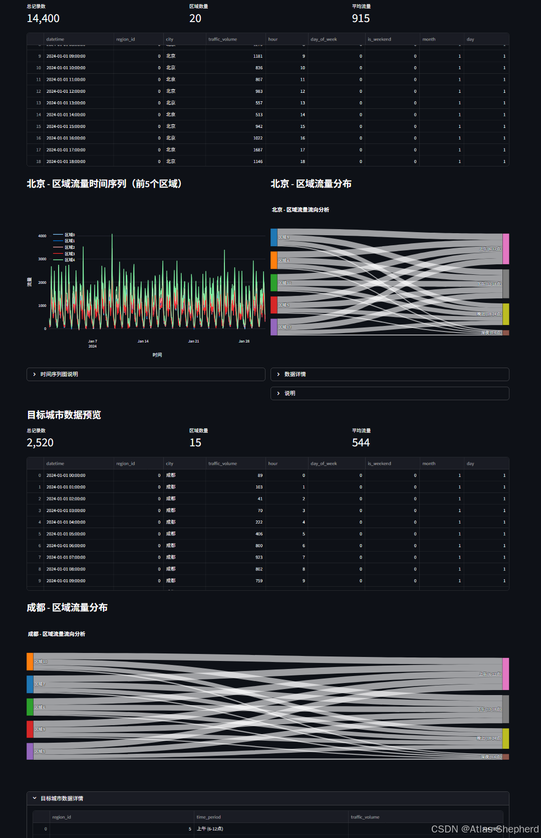
st.subheader("源城市数据预览")
col1, col2, col3 = st.columns(3)
with col1:
st.metric("总记录数", f"{len(st.session_state.source_data):,}")
with col2:
st.metric("区域数量", st.session_state.source_data['region_id'].nunique())
with col3:
st.metric("平均流量", f"{st.session_state.source_data['traffic_volume'].mean():.0f}")
st.dataframe(st.session_state.source_data.head(100), use_container_width=True)
# 创建两列布局,左侧显示时间序列图,右侧显示桑基图
col_chart1, col_chart2 = st.columns(2)
with col_chart1:
# 源城市时间序列图
st.subheader(f"{source_city} - 区域流量时间序列(前5个区域)")
fig1 = go.Figure()
for region in st.session_state.source_data['region_id'].unique()[:5]:
region_data = st.session_state.source_data[st.session_state.source_data['region_id'] == region]
fig1.add_trace(go.Scatter(
x=region_data['datetime'],
y=region_data['traffic_volume'],
mode='lines',
name=f'区域{region}',
line=dict(width=2)
))
fig1.update_layout(
xaxis_title="时间",
yaxis_title="流量",
height=500,
showlegend=True,
legend=dict(
yanchor="top",
y=0.99,
xanchor="left",
x=0.01
)
)
st.plotly_chart(fig1, use_container_width=True)
# 时间序列图解释
with st.expander("时间序列图说明"):
st.markdown("""
**时间序列图**展示了前5个区域随时间变化的流量模式:
- 可以观察到不同区域的流量变化趋势
- 识别早晚高峰时段
- 比较不同区域的流量水平
- 发现周期性变化模式
""")
with col_chart2:
# 源城市桑基图
st.subheader(f"{source_city} - 区域流量分布")
# 准备桑基图数据
nodes, source, target, value, period_flow = prepare_sankey_data(st.session_state.source_data,
top_n_regions=5)
if nodes and source and target and value:
# 创建桑基图
fig2 = go.Figure(data=[go.Sankey(
node=dict(
pad=15,
thickness=20,
line=dict(color="black", width=0.5),
label=nodes,
color=["#1f77b4", "#ff7f0e", "#2ca02c", "#d62728", "#9467bd",
"#8c564b", "#e377c2", "#7f7f7f", "#bcbd22", "#17becf"]
),
link=dict(
source=source,
target=target,
value=value
)
)])
fig2.update_layout(
title_text=f"{source_city} - 区域流量流向分析",
font_size=12,
height=500
)
st.plotly_chart(fig2, use_container_width=True)
# 显示桑基图数据表格
with st.expander("数据详情"):
st.dataframe(period_flow, use_container_width=True)
# 添加数据摘要
st.markdown("**数据摘要:**")
col_sum1, col_sum2, col_sum3 = st.columns(3)
with col_sum1:
st.metric("涉及区域数", len(period_flow['region_id'].unique()))
with col_sum2:
st.metric("时段数量", len(period_flow['time_period'].unique()))
with col_sum3:
st.metric("总连接数", len(period_flow))
else:
st.warning("无法生成桑基图数据,请确保有足够的数据")
# 桑基图解释
with st.expander("说明"):
st.markdown("""
**桑基图**展示了不同区域在一天中各时段的流量分布:
- **左侧节点**: 流量最高的5个区域
- **右侧节点**: 一天中的4个时段
- **连线宽度**: 表示流量的多少
- **颜色**: 区分不同区域和时段
**解读方法:**
1. 观察每个区域在哪些时段流量较高
2. 比较不同区域的流量分布模式
3. 识别流量集中的时段和区域
4. 发现区域间的流量差异
""")
if st.session_state.target_data is not None:
st.subheader("目标城市数据预览")
col1, col2, col3 = st.columns(3)
with col1:
st.metric("总记录数", f"{len(st.session_state.target_data):,}")
with col2:
st.metric("区域数量", st.session_state.target_data['region_id'].nunique())
with col3:
st.metric("平均流量", f"{st.session_state.target_data['traffic_volume'].mean():.0f}")
st.dataframe(st.session_state.target_data.head(50), use_container_width=True)
# 为目标城市也添加桑基图
st.subheader(f"{target_city} - 区域流量分布")
# 准备目标城市桑基图数据
target_nodes, target_source, target_target, target_value, target_period_flow = prepare_sankey_data(
st.session_state.target_data, top_n_regions=5
)
if target_nodes and target_source and target_target and target_value:
# 创建目标城市桑基图
fig3 = go.Figure(data=[go.Sankey(
node=dict(
pad=15,
thickness=20,
line=dict(color="black", width=0.5),
label=target_nodes,
color=["#1f77b4", "#ff7f0e", "#2ca02c", "#d62728", "#9467bd",
"#8c564b", "#e377c2", "#7f7f7f", "#bcbd22", "#17becf"]
),
link=dict(
source=target_source,
target=target_target,
value=target_value
)
)])
fig3.update_layout(
title_text=f"{target_city} - 区域流量流向分析",
font_size=12,
height=500
)
st.plotly_chart(fig3, use_container_width=True)
with st.expander("目标城市数据详情"):
st.dataframe(target_period_flow, use_container_width=True)
with tab2:
st.header("模型训练与迁移学习")
if st.session_state.source_data is None or st.session_state.target_data is None:
st.warning("请先生成源城市和目标城市数据")
else:
col1, col2 = st.columns(2)
with col1:
st.subheader("模型配置")
transfer_method = st.radio(
"迁移学习方法",
["直接迁移(无目标数据微调)", "微调迁移(使用少量目标数据)"],
index=1
)
fine_tune = transfer_method == "微调迁移(使用少量目标数据)"
if st.button("开始训练与迁移", type="primary"):
with st.spinner("正在进行跨城市迁移学习..."):
# 在源城市上训练
feature_cols, source_mae, source_rmse, source_r2 = st.session_state.model.train_on_source(
st.session_state.source_data
)
st.session_state.feature_cols = feature_cols
# 迁移到目标城市
target_features, target_mae, target_rmse, target_r2, source_predictions = st.session_state.model.transfer_to_target(
st.session_state.target_data, feature_cols, fine_tune=fine_tune
)
st.session_state.target_features = target_features
st.session_state.source_predictions = source_predictions
# 保存评估结果
st.session_state.evaluation_results = {
'source_city': source_city,
'target_city': target_city,
'source_metrics': {'MAE': source_mae, 'RMSE': source_rmse, 'R2': source_r2},
'target_metrics': {'MAE': target_mae, 'RMSE': target_rmse, 'R2': target_r2},
'transfer_method': transfer_method
}
with col2:
if 'evaluation_results' in st.session_state:
st.subheader("模型性能评估")
# 创建对比指标
metrics_df = pd.DataFrame({
'指标': ['MAE', 'RMSE', 'R²'],
'源城市': [
f"{st.session_state.evaluation_results['source_metrics']['MAE']:.1f}",
f"{st.session_state.evaluation_results['source_metrics']['RMSE']:.1f}",
f"{st.session_state.evaluation_results['source_metrics']['R2']:.3f}"
],
'目标城市': [
f"{st.session_state.evaluation_results['target_metrics']['MAE']:.1f}",
f"{st.session_state.evaluation_results['target_metrics']['RMSE']:.1f}",
f"{st.session_state.evaluation_results['target_metrics']['R2']:.3f}"
]
})
st.table(metrics_df)
# 性能提升计算
if st.session_state.evaluation_results['target_metrics']['R2'] > 0:
st.success(
f"迁移学习成功!目标城市R²分数: {st.session_state.evaluation_results['target_metrics']['R2']:.3f}")
# 特征重要性
if hasattr(st.session_state.model, 'target_model') and st.session_state.model.target_model is not None:
model = st.session_state.model.target_model
else:
model = st.session_state.model.source_model
feature_importance = pd.DataFrame({
'特征': st.session_state.feature_cols,
'重要性': model.feature_importances_
}).sort_values('重要性', ascending=False).head(10)
fig = px.bar(
feature_importance,
x='重要性',
y='特征',
orientation='h',
title='Top 10 重要特征'
)
st.plotly_chart(fig, use_container_width=True)
with tab3:
st.header("流量预测与分析")
if not st.session_state.model.is_fitted or 'target_features' not in st.session_state:
st.warning("请先训练模型")
else:
col1, col2 = st.columns(2)
with col1:
st.subheader("预测配置")
region_to_predict = st.selectbox(
"选择要预测的区域",
sorted(st.session_state.target_data['region_id'].unique()),
key="region_select"
)
prediction_hours = st.slider("预测小时数", 6, 72, 24, key="pred_hours")
if st.button("开始预测", type="primary"):
with st.spinner("正在生成预测..."):
# 获取选定区域的数据
region_data = st.session_state.target_features[
st.session_state.target_features['region_id'] == region_to_predict
].copy()
# 预测未来流量
future_predictions = st.session_state.model.predict_future(
region_data, st.session_state.feature_cols, hours_ahead=prediction_hours
)
if future_predictions:
st.session_state.future_predictions = future_predictions
st.session_state.region_data = region_data
with col2:
if 'future_predictions' in st.session_state:
st.subheader("预测结果")
# 创建预测时间序列
last_time = st.session_state.region_data['datetime'].iloc[-1]
future_times = [last_time + timedelta(hours=i + 1) for i in range(prediction_hours)]
predictions_df = pd.DataFrame({
'时间': future_times,
'预测流量': st.session_state.future_predictions
})
col1, col2, col3 = st.columns(3)
with col1:
avg_pred = np.mean(st.session_state.future_predictions)
st.metric("平均预测流量", f"{avg_pred:.0f}")
with col2:
max_pred = np.max(st.session_state.future_predictions)
st.metric("最大预测流量", f"{max_pred:.0f}")
with col3:
peak_hour = future_times[np.argmax(st.session_state.future_predictions)].hour
st.metric("预测高峰时段", f"{peak_hour}:00")
st.dataframe(predictions_df, use_container_width=True)
# 下载预测结果
csv = predictions_df.to_csv(index=False).encode('utf-8')
st.download_button(
label="下载预测结果(CSV)",
data=csv,
file_name=f"预测结果_{target_city}_区域{region_to_predict}.csv",
mime="text/csv"
)
with tab4:
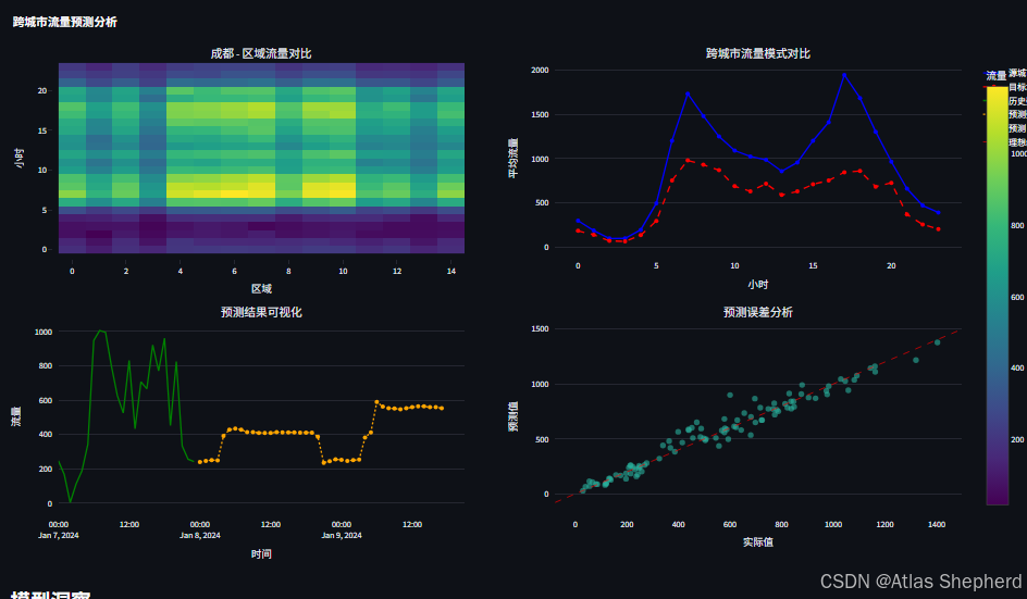
st.header("可视化分析")
if not st.session_state.model.is_fitted:
st.warning("请先训练模型")
else:
# 创建子图
fig = make_subplots(
rows=2, cols=2,
subplot_titles=(
f"{target_city} - 区域流量对比",
"跨城市流量模式对比",
"预测结果可视化",
"预测误差分析"
),
vertical_spacing=0.15,
horizontal_spacing=0.1
)
# 1. 目标城市各区域流量热图
pivot_data = st.session_state.target_data.pivot_table(
values='traffic_volume',
index='hour',
columns='region_id',
aggfunc='mean'
)
fig.add_trace(
go.Heatmap(
z=pivot_data.values,
x=pivot_data.columns,
y=pivot_data.index,
colorscale='Viridis',
colorbar=dict(title="流量")
),
row=1, col=1
)
# 2. 跨城市对比
if st.session_state.source_data is not None:
source_hourly = st.session_state.source_data.groupby('hour')['traffic_volume'].mean().reset_index()
target_hourly = st.session_state.target_data.groupby('hour')['traffic_volume'].mean().reset_index()
fig.add_trace(
go.Scatter(
x=source_hourly['hour'],
y=source_hourly['traffic_volume'],
mode='lines+markers',
name=f'源城市: {source_city}',
line=dict(color='blue', width=2)
),
row=1, col=2
)
fig.add_trace(
go.Scatter(
x=target_hourly['hour'],
y=target_hourly['traffic_volume'],
mode='lines+markers',
name=f'目标城市: {target_city}',
line=dict(color='red', width=2, dash='dash')
),
row=1, col=2
)
# 3. 预测结果
if 'future_predictions' in st.session_state and 'region_data' in st.session_state:
# 历史数据
region_hist = st.session_state.region_data.tail(24).copy()
fig.add_trace(
go.Scatter(
x=region_hist['datetime'],
y=region_hist['traffic_volume'],
mode='lines',
name='历史数据',
line=dict(color='green', width=2)
),
row=2, col=1
)
# 预测数据
last_time = region_hist['datetime'].iloc[-1]
future_times = [last_time + timedelta(hours=i + 1) for i in range(len(st.session_state.future_predictions))]
fig.add_trace(
go.Scatter(
x=future_times,
y=st.session_state.future_predictions,
mode='lines+markers',
name='预测数据',
line=dict(color='orange', width=2, dash='dot')
),
row=2, col=1
)
# 4. 误差分析
if 'source_predictions' in st.session_state and 'target_features' in st.session_state:
# 使用实际值和预测值
actual_values = st.session_state.target_features['traffic_volume'].values
predicted_values = st.session_state.source_predictions
# 限制数据量
n_points = min(100, len(actual_values))
indices = np.random.choice(len(actual_values), n_points, replace=False)
fig.add_trace(
go.Scatter(
x=actual_values[indices],
y=predicted_values[indices],
mode='markers',
name='预测 vs 实际',
marker=dict(size=8, opacity=0.6)
),
row=2, col=2
)
# 添加y=x线
min_val = min(actual_values.min(), predicted_values.min())
max_val = max(actual_values.max(), predicted_values.max())
fig.add_trace(
go.Scatter(
x=[min_val, max_val],
y=[min_val, max_val],
mode='lines',
name='理想线',
line=dict(color='red', width=1, dash='dash')
),
row=2, col=2
)
# 更新布局
fig.update_layout(
height=800,
showlegend=True,
title_text="跨城市流量预测分析"
)
fig.update_xaxes(title_text="区域", row=1, col=1)
fig.update_xaxes(title_text="小时", row=1, col=2)
fig.update_xaxes(title_text="时间", row=2, col=1)
fig.update_xaxes(title_text="实际值", row=2, col=2)
fig.update_yaxes(title_text="小时", row=1, col=1)
fig.update_yaxes(title_text="平均流量", row=1, col=2)
fig.update_yaxes(title_text="流量", row=2, col=1)
fig.update_yaxes(title_text="预测值", row=2, col=2)
st.plotly_chart(fig, use_container_width=True)
# 模型解释
st.subheader("模型洞察")
col1, col2 = st.columns(2)
with col1:
st.info("""
**迁移学习优势:**
- 利用源城市丰富数据学习通用模式
- 适应目标城市特有特征
- 减少对目标城市数据量的依赖
- 提高小数据场景下的预测精度
""")
with col2:
st.info("""
**应用场景:**
- 新城市交通规划
- 突发事件流量预测
- 节假日人流管理
- 基础设施容量规划
""")
# 页脚
st.markdown("---")
st.caption("""
**跨城市人类移动行为
""")