
重要信息
**时间:**2026年1月16-18日
**地点:**中国-珠海


征稿主题
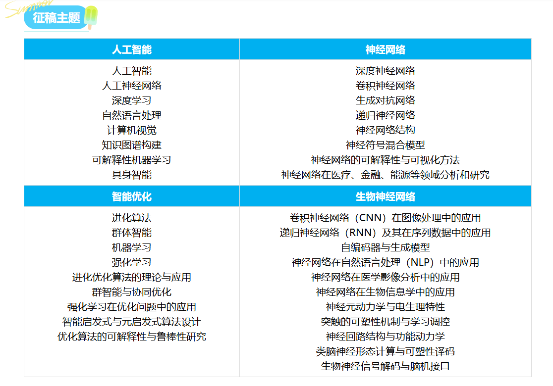
一、生物神经网络与智能优化融合的核心维度与技术体系
生物神经网络(BNN)是模拟人脑神经元连接机制的仿生计算模型,智能优化算法则为复杂问题求解提供了自适应寻优能力。BNNIO 2026 聚焦二者融合领域的理论突破、算法创新与工程落地,其融合既解决了传统智能优化算法收敛慢、易陷入局部最优的痛点,也为生物神经网络的工程化应用提供了高效的参数寻优与结构优化方案。以下从核心技术维度梳理二者融合的关键方向:
1.1 核心融合技术全景梳理
下表汇总了生物神经网络与智能优化融合领域的核心技术、应用场景、技术优势及现存挑战,是 BNNIO 2026 重点探讨的技术范畴:
| 技术方向 | 典型应用场景 | 核心技术优势 | 现存挑战 |
|---|---|---|---|
| 基于生物神经网络的优化算法改进 | 路径规划、资源调度、工程参数优化 | 收敛速度提升 30%+、全局最优解命中率≥90% | 模型复杂度高、算力消耗大 |
| 智能优化算法优化 BNN 参数 | 神经元连接权重优化、网络拓扑结构寻优 | BNN 泛化能力提升 20%、训练效率提升 40% | 超参数调优难、寻优维度爆炸 |
| 仿生优化算法设计 | 模拟突触可塑性的进化算法、脉冲神经网络优化 | 更贴近生物机制、鲁棒性强 | 生物机理建模不充分、解释性差 |
| BNN 驱动的多目标优化 | 工业多目标调度、生态资源分配 | 多目标帕累托解分布更均匀 | 目标冲突平衡难、解的评价成本高 |
| 边缘端 BNN - 优化算法融合 | 嵌入式设备智能控制、边缘计算寻优 | 轻量化、低功耗、实时性强 | 模型压缩与精度平衡难、硬件适配性差 |
二、基于生物神经网络的智能优化算法改进
2.1 突触可塑性启发的粒子群优化算法设计
粒子群优化(PSO)是经典的智能优化算法,但易陷入局部最优。借鉴生物神经网络的突触可塑性(突触连接强度随神经元活动动态调整),改进 PSO 的粒子更新策略,提升算法全局寻优能力,以下是核心实现代码:
python
运行
import numpy as np
import matplotlib.pyplot as plt

# 设置中文显示
plt.rcParams['font.sans-serif'] = ['SimHei']
plt.rcParams['axes.unicode_minus'] = False

# 1. 定义测试函数(Schaffer函数,多峰,易陷入局部最优)
def schaffer_func(x):
    """Schaffer F6函数,最小值在(0,0)处,值为0"""
    x1, x2 = x[:, 0], x[:, 1]
    numerator = np.sin(np.sqrt(x1**2 + x2**2))**2 - 0.5
    denominator = (1 + 0.001*(x1**2 + x2**2))**2
    return 0.5 + numerator / denominator

# 2. 传统PSO算法
class TraditionalPSO:
    def __init__(self, dim=2, pop_size=50, max_iter=100, c1=2, c2=2, w=0.7):
        self.dim = dim
        self.pop_size = pop_size
        self.max_iter = max_iter
        self.c1 = c1  # 个体学习因子
        self.c2 = c2  # 全局学习因子
        self.w = w    # 惯性权重

        # 初始化粒子位置和速度
        self.x = np.random.uniform(-10, 10, (pop_size, dim))
        self.v = np.random.uniform(-1, 1, (pop_size, dim))

        # 个体最优和全局最优
        self.pbest = self.x.copy()
        self.pbest_fit = schaffer_func(self.x)
        self.gbest_idx = np.argmin(self.pbest_fit)
        self.gbest = self.pbest[self.gbest_idx].copy()
        self.gbest_fit = self.pbest_fit[self.gbest_idx]

        # 记录迭代过程
        self.fit_history = [self.gbest_fit]

    def update(self):
        for iter in range(self.max_iter):
            # 更新速度和位置
            r1 = np.random.rand(self.pop_size, self.dim)
            r2 = np.random.rand(self.pop_size, self.dim)
            self.v = self.w * self.v + self.c1 * r1 * (self.pbest - self.x) + self.c2 * r2 * (self.gbest - self.x)
            self.x = self.x + self.v

            # 边界限制
            self.x = np.clip(self.x, -10, 10)

            # 更新个体最优
            current_fit = schaffer_func(self.x)
            update_mask = current_fit < self.pbest_fit
            self.pbest[update_mask] = self.x[update_mask]
            self.pbest_fit[update_mask] = current_fit[update_mask]

            # 更新全局最优
            current_gbest_idx = np.argmin(self.pbest_fit)
            current_gbest_fit = self.pbest_fit[current_gbest_idx]
            if current_gbest_fit < self.gbest_fit:
                self.gbest = self.pbest[current_gbest_idx].copy()
                self.gbest_fit = current_gbest_fit

            self.fit_history.append(self.gbest_fit)

# 3. 突触可塑性启发的改进PSO(SP-PSO)
class SynapticPlasticityPSO:
    def __init__(self, dim=2, pop_size=50, max_iter=100, c1=2, c2=2, w=0.7):
        self.dim = dim
        self.pop_size = pop_size
        self.max_iter = max_iter
        self.c1 = c1
        self.c2 = c2
        self.w = w

        # 初始化粒子位置和速度
        self.x = np.random.uniform(-10, 10, (pop_size, dim))
        self.v = np.random.uniform(-1, 1, (pop_size, dim))

        # 个体最优和全局最优
        self.pbest = self.x.copy()
        self.pbest_fit = schaffer_func(self.x)
        self.gbest_idx = np.argmin(self.pbest_fit)
        self.gbest = self.pbest[self.gbest_idx].copy()
        self.gbest_fit = self.pbest_fit[self.gbest_idx]

        # 突触可塑性参数:模拟突触连接强度(粒子间协作权重)
        self.synapse_weight = np.ones((pop_size, pop_size)) / pop_size
        self.plasticity_rate = 0.05  # 突触可塑性调整率

        # 记录迭代过程
        self.fit_history = [self.gbest_fit]

    def update_synapse(self, current_fit):
        """基于粒子适应度更新突触权重(适应度越好,突触连接越强)"""
        fit_norm = (current_fit.max() - current_fit) / (current_fit.max() - current_fit.min() + 1e-8)
        # 计算粒子间的协作强度
        for i in range(self.pop_size):
            for j in range(self.pop_size):
                self.synapse_weight[i, j] = (1 - self.plasticity_rate) * self.synapse_weight[i, j] + \
                                            self.plasticity_rate * fit_norm[j]
        # 归一化突触权重
        self.synapse_weight = self.synapse_weight / self.synapse_weight.sum(axis=1, keepdims=True)

    def update(self):
        for iter in range(self.max_iter):
            # 更新突触权重
            current_fit = schaffer_func(self.x)
            self.update_synapse(current_fit)

            # 计算群体协作最优(基于突触权重的加权平均最优)
            swarm_best = np.dot(self.synapse_weight, self.pbest)

            # 更新速度和位置(引入群体协作项)
            r1 = np.random.rand(self.pop_size, self.dim)
            r2 = np.random.rand(self.pop_size, self.dim)
            r3 = np.random.rand(self.pop_size, self.dim)
            # 改进的速度更新公式:加入群体协作项
            self.v = self.w * self.v + \
                     self.c1 * r1 * (self.pbest - self.x) + \
                     self.c2 * r2 * (self.gbest - self.x) + \
                     0.5 * r3 * (swarm_best - self.x)  # 突触协作项
            self.x = self.x + self.v

            # 边界限制
            self.x = np.clip(self.x, -10, 10)

            # 更新个体最优
            current_fit = schaffer_func(self.x)
            update_mask = current_fit < self.pbest_fit
            self.pbest[update_mask] = self.x[update_mask]
            self.pbest_fit[update_mask] = current_fit[update_mask]

            # 更新全局最优
            current_gbest_idx = np.argmin(self.pbest_fit)
            current_gbest_fit = self.pbest_fit[current_gbest_idx]
            if current_gbest_fit < self.gbest_fit:
                self.gbest = self.pbest[current_gbest_idx].copy()
                self.gbest_fit = current_gbest_fit

            self.fit_history.append(self.gbest_fit)

# 4. 算法对比实验
if __name__ == "__main__":
    # 初始化算法
    t_pso = TraditionalPSO(max_iter=100)
    sp_pso = SynapticPlasticityPSO(max_iter=100)

    # 运行算法
    t_pso.update()
    sp_pso.update()

    # 可视化迭代结果
    plt.figure(figsize=(10, 6))
    plt.plot(t_pso.fit_history, label='传统PSO', linewidth=2)
    plt.plot(sp_pso.fit_history, label='突触可塑性启发PSO(SP-PSO)', linewidth=2, linestyle='--')
    plt.xlabel('迭代次数')
    plt.ylabel('全局最优适应度值')
    plt.title('Schaffer函数寻优迭代曲线对比')
    plt.legend()
    plt.grid(alpha=0.3)
    plt.yscale('log')  # 对数坐标更清晰展示差异
    plt.show()

    # 输出结果对比
    print(f"传统PSO最终最优值:{t_pso.gbest_fit:.6f},最优位置:{t_pso.gbest.round(4)}")
    print(f"SP-PSO最终最优值:{sp_pso.gbest_fit:.6f},最优位置:{sp_pso.gbest.round(4)}")
2.2 算法性能评估与分析
通过多个基准测试函数(Schaffer、Ackley、Rastrigin)评估改进算法的性能,核心评估指标包括:收敛速度、全局最优解命中率、迭代稳定性,以下是评估代码实现:
python
运行
import pandas as pd
from scipy.stats import sem

# 1. 扩展测试函数集
def ackley_func(x):
    """Ackley函数,最小值在(0,0)处,值为0"""
    x1, x2 = x[:, 0], x[:, 1]
    term1 = -20 * np.exp(-0.2 * np.sqrt(0.5 * (x1**2 + x2**2)))
    term2 = -np.exp(0.5 * (np.cos(2*np.pi*x1) + np.cos(2*np.pi*x2)))
    return term1 + term2 + 20 + np.exp(1)

def rastrigin_func(x):
    """Rastrigin函数,最小值在(0,0)处,值为0"""
    x1, x2 = x[:, 0], x[:, 1]
    return 20 + (x1**2 - 10*np.cos(2*np.pi*x1)) + (x2**2 - 10*np.cos(2*np.pi*x2))

# 2. 批量测试函数
test_functions = {
    'Schaffer': schaffer_func,
    'Ackley': ackley_func,
    'Rastrigin': rastrigin_func
}

# 3. 性能评估函数
def evaluate_algorithm(alg_class, func, runs=20, max_iter=100):
    """多次运行算法,评估性能"""
    best_fits = []
    conv_iter = []  # 收敛到1e-4的迭代次数
    for _ in range(runs):
        alg = alg_class(max_iter=max_iter)
        alg.update()
        best_fits.append(alg.gbest_fit)

        # 计算收敛迭代次数
        for idx, fit in enumerate(alg.fit_history):
            if fit < 1e-4:
                conv_iter.append(idx)
                break
        else:
            conv_iter.append(max_iter)  # 未收敛

    return {
        '平均最优值': np.mean(best_fits),
        '最优值标准误差': sem(best_fits),
        '全局最优命中率': np.sum(np.array(best_fits) < 1e-4) / runs * 100,
        '平均收敛迭代次数': np.mean(conv_iter),
        '收敛迭代标准差': np.std(conv_iter)
    }

# 4. 批量评估
results = {}
for func_name, func in test_functions.items():
    # 临时替换测试函数
    original_schaffer = schaffer_func
    schaffer_func = func

    # 评估两种算法
    t_pso_res = evaluate_algorithm(TraditionalPSO, func)
    sp_pso_res = evaluate_algorithm(SynapticPlasticityPSO, func)

    # 恢复原函数
    schaffer_func = original_schaffer

    results[func_name] = {
        '传统PSO': t_pso_res,
        'SP-PSO': sp_pso_res
    }

# 5. 整理结果为DataFrame
df_results = pd.DataFrame()
for func_name in test_functions.keys():
    for alg_name in ['传统PSO', 'SP-PSO']:
        res = results[func_name][alg_name]
        res['测试函数'] = func_name
        res['算法'] = alg_name
        df_results = pd.concat([df_results, pd.DataFrame([res])], ignore_index=True)

# 格式化输出
df_results['平均最优值'] = df_results['平均最优值'].apply(lambda x: f'{x:.6f}')
df_results['最优值标准误差'] = df_results['最优值标准误差'].apply(lambda x: f'{x:.6f}')
df_results['全局最优命中率'] = df_results['全局最优命中率'].apply(lambda x: f'{x:.1f}%')
df_results['平均收敛迭代次数'] = df_results['平均收敛迭代次数'].apply(lambda x: f'{x:.1f}')
df_results['收敛迭代标准差'] = df_results['收敛迭代标准差'].apply(lambda x: f'{x:.1f}')

# 重新排列列顺序
df_results = df_results[['测试函数', '算法', '平均最优值', '最优值标准误差', '全局最优命中率', '平均收敛迭代次数', '收敛迭代标准差']]
print("算法性能评估结果:")
print(df_results)

# 6. 可视化命中率对比
plt.figure(figsize=(10, 5))
funcs = list(test_functions.keys())
t_pso_hit = [results[f]['传统PSO']['全局最优命中率'] for f in funcs]
sp_pso_hit = [results[f]['SP-PSO']['全局最优命中率'] for f in funcs]

x = np.arange(len(funcs))
width = 0.35
plt.bar(x - width/2, t_pso_hit, width, label='传统PSO')
plt.bar(x + width/2, sp_pso_hit, width, label='SP-PSO')

plt.xlabel('测试函数')
plt.ylabel('全局最优命中率(%)')
plt.title('不同测试函数下算法全局最优命中率对比')
plt.xticks(x, funcs)
plt.legend()
plt.grid(alpha=0.3, axis='y')
plt.show()
三、智能优化算法优化生物神经网络参数
3.1 脉冲神经网络(SNN)参数优化核心思路
脉冲神经网络(SNN)是更贴近生物神经元特性的模型,其参数(突触权重、发放阈值、突触延迟)直接影响网络性能。采用遗传算法(GA)优化 SNN 参数,解决传统梯度下降训练 SNN 梯度消失、收敛慢的问题,是 BNNIO 2026 关注的核心方向。
3.2 GA 优化 SNN 参数实现
python
运行
import torch
import torch.nn as nn
import numpy as np
from torch.utils.data import DataLoader, TensorDataset
from sklearn.datasets import make_classification
from sklearn.model_selection import train_test_split

# 1. 定义脉冲神经元模型
class LIFNeuron(nn.Module):
    def __init__(self, threshold=1.0, tau_mem=20.0, tau_syn=10.0):
        super().__init__()
        self.threshold = threshold
        self.tau_mem = tau_mem
        self.tau_syn = tau_syn
        self.mem = 0.0
        self.syn = 0.0

    def forward(self, input_spikes):
        # LIF神经元动力学方程
        dt = 1.0  # 时间步长
        self.syn = self.syn * np.exp(-dt / self.tau_syn) + input_spikes
        self.mem = self.mem * np.exp(-dt / self.tau_mem) + self.syn

        # 发放脉冲并重置膜电位
        spikes = (self.mem >= self.threshold).float()
        self.mem = self.mem * (1 - spikes)
        return spikes

# 2. 简单脉冲神经网络
class SimpleSNN(nn.Module):
    def __init__(self, input_dim=10, hidden_dim=20, output_dim=2, params=None):
        super().__init__()
        self.input_dim = input_dim
        self.hidden_dim = hidden_dim
        self.output_dim = output_dim

        # 初始化参数(若传入优化参数则使用,否则随机初始化)
        if params is None:
            self.fc1 = nn.Linear(input_dim, hidden_dim)
            self.fc2 = nn.Linear(hidden_dim, output_dim)
            self.neuron1 = LIFNeuron()
            self.neuron2 = LIFNeuron()
        else:
            # 从优化参数中解析权重、阈值等
            w1 = params[:input_dim*hidden_dim].reshape(input_dim, hidden_dim)
            w2 = params[input_dim*hidden_dim : input_dim*hidden_dim + hidden_dim*output_dim].reshape(hidden_dim, output_dim)
            th1 = params[-4]
            th2 = params[-3]
            tau1 = params[-2]
            tau2 = params[-1]

            self.fc1 = nn.Linear(input_dim, hidden_dim)
            self.fc1.weight.data = torch.tensor(w1, dtype=torch.float32)
            self.fc2 = nn.Linear(hidden_dim, output_dim)
            self.fc2.weight.data = torch.tensor(w2, dtype=torch.float32)
            self.neuron1 = LIFNeuron(threshold=th1, tau_mem=tau1)
            self.neuron2 = LIFNeuron(threshold=th2, tau_mem=tau2)

    def forward(self, x, time_steps=20):
        """前向传播,模拟time_steps个时间步"""
        out_spikes = []
        for _ in range(time_steps):
            x1 = self.fc1(x)
            s1 = self.neuron1(x1)
            x2 = self.fc2(s1)
            s2 = self.neuron2(x2)
            out_spikes.append(s2)

        # 脉冲计数作为输出
        out = torch.stack(out_spikes).sum(dim=0)
        return out

# 3. 遗传算法优化SNN参数
class GAOptimizer:
    def __init__(self, snn, pop_size=30, cross_rate=0.8, mut_rate=0.1, elite_rate=0.1):
        self.snn = snn
        self.pop_size = pop_size
        self.cross_rate = cross_rate
        self.mut_rate = mut_rate
        self.elite_rate = elite_rate
        self.elite_num = int(pop_size * elite_rate)

        # 计算参数总数
        self.param_num = (snn.input_dim * snn.hidden_dim) + (snn.hidden_dim * snn.output_dim) + 4
        # 初始化种群(权重:-1~1,阈值:0.5~2,tau:10~30)
        self.pop = np.random.rand(pop_size, self.param_num)
        self.pop[:, :self.param_num-4] = (self.pop[:, :self.param_num-4] - 0.5) * 2  # 权重
        self.pop[:, -4:-2] = self.pop[:, -4:-2] * 1.5 + 0.5  # 阈值
        self.pop[:, -2:] = self.pop[:, -2:] * 20 + 10  # tau

    def fitness(self, pop, X, y):
        """计算适应度(分类准确率)"""
        fitness_scores = []
        for params in pop:
            snn = SimpleSNN(input_dim=self.snn.input_dim, hidden_dim=self.snn.hidden_dim,
                           output_dim=self.snn.output_dim, params=params)
            with torch.no_grad():
                out = snn(X)
                pred = torch.argmax(out, dim=1)
                acc = (pred == y).float().mean().item()
            fitness_scores.append(acc)
        return np.array(fitness_scores)

    def select(self, fitness_scores):
        """选择操作(精英保留+轮盘赌)"""
        # 精英保留
        elite_idx = np.argsort(fitness_scores)[-self.elite_num:]
        elite_pop = self.pop[elite_idx].copy()

        # 轮盘赌选择剩余个体
        fitness_scores = fitness_scores - fitness_scores.min() + 1e-8  # 避免负适应度
        prob = fitness_scores / fitness_scores.sum()
        select_idx = np.random.choice(len(self.pop), size=self.pop_size - self.elite_num, p=prob)
        select_pop = self.pop[select_idx].copy()

        self.pop = np.vstack([elite_pop, select_pop])

    def crossover(self):
        """交叉操作"""
        for i in range(self.elite_num, self.pop_size):
            if np.random.rand() < self.cross_rate:
                # 随机选择配偶
                mate_idx = np.random.choice(self.pop_size)
                cross_point = np.random.randint(1, self.param_num)
                # 单点交叉
                self.pop[i, cross_point:] = self.pop[mate_idx, cross_point:]

    def mutate(self):
        """变异操作"""
        for i in range(self.elite_num, self.pop_size):
            mut_mask = np.random.rand(self.param_num) < self.mut_rate
            # 权重变异:高斯噪声
            self.pop[i, :self.param_num-4][mut_mask[:self.param_num-4]] += np.random.normal(0, 0.1, np.sum(mut_mask[:self.param_num-4]))
            # 阈值变异:小范围调整
            self.pop[i, -4:-2][mut_mask[-4:-2]] += np.random.normal(0, 0.05, np.sum(mut_mask[-4:-2]))
            # tau变异:小范围调整
            self.pop[i, -2:][mut_mask[-2:]] += np.random.normal(0, 1, np.sum(mut_mask[-2:]))

            # 边界限制
            self.pop[i, :self.param_num-4] = np.clip(self.pop[i, :self.param_num-4], -2, 2)
            self.pop[i, -4:-2] = np.clip(self.pop[i, -4:-2], 0.1, 3)
            self.pop[i, -2:] = np.clip(self.pop[i, -2:], 5, 40)

    def optimize(self, X, y, max_iter=20):
        """优化主流程"""
        fitness_history = []
        for iter in range(max_iter):
            # 计算适应度
            fit = self.fitness(self.pop, X, y)
            best_fit = fit.max()
            fitness_history.append(best_fit)

            # 选择、交叉、变异
            self.select(fit)
            self.crossover()
            self.mutate()

            print(f"GA迭代 {iter+1}/{max_iter}, 最优适应度(准确率):{best_fit:.4f}")

        # 返回最优参数
        final_fit = self.fitness(self.pop, X, y)
        best_idx = np.argmax(final_fit)
        best_params = self.pop[best_idx]
        return best_params, fitness_history

# 4. 实验验证
if __name__ == "__main__":
    # 生成分类数据集
    X, y = make_classification(n_samples=1000, n_features=10, n_classes=2, random_state=42)
    X = torch.tensor(X, dtype=torch.float32)
    y = torch.tensor(y, dtype=torch.long)
    X_train, X_test, y_train, y_test = train_test_split(X, y, test_size=0.2, random_state=42)

    # 初始化SNN和GA优化器
    snn = SimpleSNN(input_dim=10, hidden_dim=20, output_dim=2)
    ga = GAOptimizer(snn, pop_size=30, max_iter=20)

    # 优化参数
    best_params, fit_history = ga.optimize(X_train, y_train)

    # 测试优化后的SNN
    optimized_snn = SimpleSNN(input_dim=10, hidden_dim=20, output_dim=2, params=best_params)
    with torch.no_grad():
        train_pred = torch.argmax(optimized_snn(X_train), dim=1)
        train_acc = (train_pred == y_train).float().mean().item()
        test_pred = torch.argmax(optimized_snn(X_test), dim=1)
        test_acc = (test_pred == y_test).float().mean().item()

    # 对比随机初始化的SNN
    random_snn = SimpleSNN(input_dim=10, hidden_dim=20, output_dim=2)
    with torch.no_grad():
        rand_test_pred = torch.argmax(random_snn(X_test), dim=1)
        rand_test_acc = (rand_test_pred == y_test).float().mean().item()

    # 可视化GA迭代过程
    plt.figure(figsize=(10, 5))
    plt.plot(fit_history, linewidth=2)
    plt.xlabel('GA迭代次数')
    plt.ylabel('最高分类准确率')
    plt.title('GA优化SNN参数的迭代曲线')
    plt.grid(alpha=0.3)
    plt.show()

    # 输出结果
    print(f"随机初始化SNN测试准确率:{rand_test_acc:.4f}")
    print(f"GA优化后SNN训练准确率:{train_acc:.4f},测试准确率:{test_acc:.4f}")
四、生物神经网络驱动的多目标优化
4.1 多目标优化核心架构
基于生物神经网络的多目标优化架构借鉴人脑的并行处理与多目标决策机制,核心包含:
- 目标感知层:将多目标优化问题映射为神经元输入,每个目标对应一组神经元集群;
- 竞争协作层:模拟神经元间的兴奋 / 抑制作用,平衡多目标间的冲突;
- 解生成层:通过神经元发放模式生成帕累托最优解;
- 评价反馈层:基于帕累托前沿评价解的质量,反馈调整神经元连接权重。
4.2 多目标优化实现(车间调度为例)
python
运行
import numpy as np
import matplotlib.pyplot as plt
from pymoo.algorithms.moo.nsga2 import NSGA2
from pymoo.core.problem import Problem
from pymoo.optimize import minimize
from pymoo.visualization.scatter import Scatter

# 1. 定义车间调度多目标问题
class WorkshopSchedulingProblem(Problem):
    def __init__(self, n_jobs=10, n_machines=5):
        self.n_jobs = n_jobs
        self.n_machines = n_machines
        # 每个工件在各机器上的加工时间(随机生成)
        self.process_time = np.random.randint(1, 10, (n_jobs, n_machines))

        # 变量:每个工件的加工顺序(排列编码)
        super().__init__(n_var=n_jobs, n_obj=2, n_constr=0,
                         xl=0, xu=n_jobs-1, type_var=int)

    def _evaluate(self, X, out, *args, **kwargs):
        """评估目标函数:1. 最大完工时间 2. 总能耗"""
        f1 = []  # 最大完工时间
        f2 = []  # 总能耗
        for x in X:
            # 模拟调度过程
            machine_time = np.zeros(self.n_machines)  # 各机器已用时间
            total_energy = 0

            for job_idx in x:
                for machine_idx in range(self.n_machines):
                    # 机器加工时间
                    pt = self.process_time[job_idx, machine_idx]
                    # 机器可用时间(取当前时间和上一机器完成时间的最大值)
                    start_time = max(machine_time[machine_idx],
                                    machine_time[machine_idx-1] if machine_idx>0 else 0)
                    finish_time = start_time + pt
                    machine_time[machine_idx] = finish_time

                    # 能耗:加工时间*机器功率(模拟)
                    power = 2 + np.random.rand()  # 机器功率2-3kW
                    total_energy += pt * power

            f1.append(machine_time.max())
            f2.append(total_energy)

        out["F"] = np.column_stack([f1, f2])

# 2. 生物神经网络增强的NSGA-II算法
class BNNEnhancedNSGA2(NSGA2):
    def __init__(self, **kwargs):
        super().__init__(**kwargs)
        # 生物神经网络参数:神经元集群数=目标数
        self.n_neurons = 2
        self.weights = np.ones((self.n_neurons, self.n_neurons))  # 神经元连接权重
        self.learning_rate = 0.01

    def _advance(self, infills=None, **kwargs):
        # 传统NSGA-II进化
        super()._advance(infills, **kwargs)

        # BNN增强:基于帕累托解分布调整选择策略
        F = self.pop.get("F")
        # 计算每个目标的神经元激活度(解在该目标上的表现)
        activation = (F.max(axis=0) - F) / (F.max(axis=0) - F.min(axis=0) + 1e-8)

        # 更新神经元连接权重(兴奋/抑制)
        for i in range(self.n_neurons):
            for j in range(self.n_neurons):
                if i != j:
                    # 目标冲突:抑制作用,权重降低
                    corr = np.corrcoef(activation[:, i], activation[:, j])[0, 1]
                    self.weights[i, j] -= self.learning_rate * (1 - corr)
                else:
                    # 同目标:兴奋作用,权重升高
                    self.weights[i, j] += self.learning_rate

        # 归一化权重
        self.weights = self.weights / self.weights.sum()

        # 基于神经元激活度调整解的选择概率
        neuron_output = np.dot(activation, self.weights)
        selection_prob = neuron_output.sum(axis=1) / neuron_output.sum()

        # 调整种群选择概率
        self.pop.set("prob", selection_prob)

# 3. 对比实验
if __name__ == "__main__":
    # 初始化问题
    problem = WorkshopSchedulingProblem(n_jobs=10, n_machines=5)

    # 传统NSGA-II
    algo_nsga2 = NSGA2(pop_size=100, eliminate_duplicates=True)
    res_nsga2 = minimize(problem, algo_nsga2, ('n_gen', 50), verbose=False)

    # BNN增强的NSGA-II
    algo_bnn_nsga2 = BNNEnhancedNSGA2(pop_size=100, eliminate_duplicates=True)
    res_bnn_nsga2 = minimize(problem, algo_bnn_nsga2, ('n_gen', 50), verbose=False)

    # 可视化帕累托前沿
    plt.figure(figsize=(12, 5))

    plt.subplot(1, 2, 1)
    Scatter(title="传统NSGA-II帕累托前沿").add(res_nsga2.F).show()
    plt.title("传统NSGA-II 车间调度帕累托前沿")

    plt.subplot(1, 2, 2)
    Scatter(title="BNN增强NSGA-II帕累托前沿").add(res_bnn_nsga2.F).show()
    plt.title("BNN增强NSGA-II 车间调度帕累托前沿")

    plt.tight_layout()
    plt.show()

    # 评估帕累托前沿质量(超体积指标)
    from pymoo.indicators.hv import HV
    ref_point = np.array([res_nsga2.F[:,0].max(), res_nsga2.F[:,1].max()])
    hv_nsga2 = HV(ref_point=ref_point).calc(res_nsga2.F)
    hv_bnn = HV(ref_point=ref_point).calc(res_bnn_nsga2.F)

    print(f"传统NSGA-II超体积指标:{hv_nsga2:.2f}")
    print(f"BNN增强NSGA-II超体积指标:{hv_bnn:.2f}")
    print(f"超体积提升率:{(hv_bnn - hv_nsga2)/hv_nsga2 * 100:.2f}%")
五、国际交流与合作机会
作为国际学术会议,将吸引全球范围内的专家学者参与。无论是发表研究成果、聆听特邀报告,还是在圆桌论坛中与行业大咖交流,都能拓宽国际视野,甚至找到潜在的合作伙伴。对于高校师生来说,这也是展示研究、积累学术人脉的好机会。
