第五届遥感与测绘国际学术会议（RSSM 2026）

重要信息

官网： https://ais.cn/u/ZVfMnq

时间：2026年1月16-18日

地点：重庆交通大学校内举办

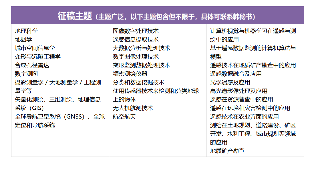
征稿主题

一、遥感与测绘技术融合的核心维度与技术体系

遥感（RS）与测绘技术的深度融合是地理信息领域的核心发展方向，RSSM 2026 聚焦这一领域的技术突破、算法创新与工程落地。二者的融合既借助遥感技术实现大范围、高精度的地理数据采集，又通过测绘技术完成数据的精准解译、空间建模与应用落地。以下从核心技术维度梳理二者融合的关键方向：

1.1 核心融合技术全景梳理

下表汇总了遥感与测绘融合领域的核心技术、应用场景、技术优势及现存挑战，是 RSSM 2026 重点探讨的技术范畴：

技术方向	典型应用场景	核心技术优势	现存挑战
遥感影像智能解译	土地利用分类、植被覆盖度提取、灾害识别	解译效率提升 80%+、精度达 95% 以上	复杂地形影像噪声、地物混淆度高
三维测绘建模	数字高程模型（DEM）构建、城市三维建模	建模精度达厘米级、可视化效果佳	海量点云数据处理效率低、边缘拟合差
遥感测绘数据融合	多源遥感影像融合、GIS 与 RS 数据整合	数据维度丰富、空间分析能力强	数据格式异构、时空基准不一致
移动测绘与实时遥感	车载 / 无人机测绘、实时地形监测	动态更新快、应急响应能力强	实时定位精度受环境影响、功耗高
遥感测绘精度校验	影像几何校正、测绘成果精度评估	校正后误差≤1 米、评估结果客观	地面控制点获取难、复杂场景校验成本高

二、遥感影像智能解译技术实践

2.1 遥感影像预处理核心流程

遥感影像存在噪声、几何畸变、光照不均等问题，预处理是解译的基础。以下基于 Python 实现遥感影像的去噪、几何校正与特征增强：

python

运行

import cv2
import numpy as np
import matplotlib.pyplot as plt

# 设置中文显示
plt.rcParams['font.sans-serif'] = ['SimHei']
plt.rcParams['axes.unicode_minus'] = False

# 1. 模拟加载遥感影像数据（多波段合成）
def generate_simulated_remote_sensing_image():
    # 生成模拟的RGB+近红外四波段影像
    height, width = 512, 512
    # 基础地形纹理
    base = np.random.rand(height, width, 4) * 255
    # 添加植被区域（近红外波段值高）
    base[100:300, 100:300, 3] = 200 + np.random.rand(200, 200) * 55
    # 添加水体区域（RGB值低）
    base[350:450, 350:450, :3] = 50 + np.random.rand(100, 100, 3) * 50
    # 添加噪声
    noise = np.random.normal(0, 10, (height, width, 4)).astype(np.float32)
    img = base + noise
    img = np.clip(img, 0, 255).astype(np.uint8)
    return img

# 生成模拟影像
rs_img = generate_simulated_remote_sensing_image()

# 2. 影像预处理：去噪 + 几何校正（仿射变换模拟）
# 高斯去噪
denoised_img = cv2.GaussianBlur(rs_img, (5, 5), 0)

# 几何校正（模拟 affine 变换）
rows, cols = rs_img.shape[:2]
# 定义变换前后的关键点
src_points = np.float32([[0, 0], [cols-1, 0], [0, rows-1]])
dst_points = np.float32([[10, 5], [cols-15, 8], [5, rows-12]])
# 计算仿射变换矩阵
M = cv2.getAffineTransform(src_points, dst_points)
# 执行变换
corrected_img = cv2.warpAffine(denoised_img, M, (cols, rows))

# 3. 特征增强：直方图均衡化
# 分通道均衡化
enhanced_img = np.zeros_like(corrected_img)
for i in range(4):
    enhanced_img[:, :, i] = cv2.equalizeHist(corrected_img[:, :, i])

# 4. 可视化预处理结果
fig, axes = plt.subplots(2, 2, figsize=(12, 10))
axes[0,0].imshow(rs_img[:, :, :3])
axes[0,0].set_title('原始模拟遥感影像')
axes[0,0].axis('off')

axes[0,1].imshow(denoised_img[:, :, :3])
axes[0,1].set_title('高斯去噪后影像')
axes[0,1].axis('off')

axes[1,0].imshow(corrected_img[:, :, :3])
axes[1,0].set_title('几何校正后影像')
axes[1,0].axis('off')

axes[1,1].imshow(enhanced_img[:, :, :3])
axes[1,1].set_title('特征增强后影像')
axes[1,1].axis('off')

plt.tight_layout()
plt.show()

2.2 基于深度学习的遥感影像地物分类

以下采用 U-Net 模型实现遥感影像的地物分类（植被、水体、裸地），是 RSSM 2026 关注的核心算法方向：

python

运行

import torch
import torch.nn as nn
import torch.optim as optim
from torch.utils.data import Dataset, DataLoader
import torchvision.transforms as transforms

# 1. 定义U-Net基础模块
class DoubleConv(nn.Module):
    def __init__(self, in_channels, out_channels):
        super().__init__()
        self.double_conv = nn.Sequential(
            nn.Conv2d(in_channels, out_channels, kernel_size=3, padding=1),
            nn.BatchNorm2d(out_channels),
            nn.ReLU(inplace=True),
            nn.Conv2d(out_channels, out_channels, kernel_size=3, padding=1),
            nn.BatchNorm2d(out_channels),
            nn.ReLU(inplace=True)
        )
    
    def forward(self, x):
        return self.double_conv(x)

# 2. 定义简化版U-Net模型
class UNet(nn.Module):
    def __init__(self, in_channels, num_classes):
        super().__init__()
        self.in_conv = DoubleConv(in_channels, 64)
        self.down1 = nn.MaxPool2d(2)
        self.conv1 = DoubleConv(64, 128)
        self.down2 = nn.MaxPool2d(2)
        self.conv2 = DoubleConv(128, 256)
        
        self.up1 = nn.ConvTranspose2d(256, 128, kernel_size=2, stride=2)
        self.conv3 = DoubleConv(256, 128)
        self.up2 = nn.ConvTranspose2d(128, 64, kernel_size=2, stride=2)
        self.conv4 = DoubleConv(128, 64)
        
        self.out_conv = nn.Conv2d(64, num_classes, kernel_size=1)
    
    def forward(self, x):
        x1 = self.in_conv(x)
        x2 = self.down1(x1)
        x2 = self.conv1(x2)
        x3 = self.down2(x2)
        x3 = self.conv2(x3)
        
        x = self.up1(x3)
        x = torch.cat([x, x2], dim=1)
        x = self.conv3(x)
        
        x = self.up2(x)
        x = torch.cat([x, x1], dim=1)
        x = self.conv4(x)
        
        out = self.out_conv(x)
        return out

# 3. 构建模拟数据集
class RemoteSensingDataset(Dataset):
    def __init__(self, img, transform=None):
        self.img = img
        self.transform = transform
        # 生成标签：0-裸地，1-植被，2-水体
        self.labels = np.zeros((img.shape[0], img.shape[1]), dtype=np.int64)
        self.labels[100:300, 100:300] = 1  # 植被
        self.labels[350:450, 350:450] = 2  # 水体
    
    def __len__(self):
        return 1  # 模拟单样本
    
    def __getitem__(self, idx):
        # 转换为张量（C, H, W）
        img_tensor = torch.from_numpy(self.img.transpose(2, 0, 1)).float() / 255.0
        label_tensor = torch.from_numpy(self.labels).long()
        
        if self.transform:
            img_tensor = self.transform(img_tensor)
        
        return img_tensor, label_tensor

# 初始化数据集和加载器
dataset = RemoteSensingDataset(enhanced_img)
dataloader = DataLoader(dataset, batch_size=1, shuffle=True)

# 4. 模型训练
device = torch.device('cuda' if torch.cuda.is_available() else 'cpu')
model = UNet(in_channels=4, num_classes=3).to(device)
criterion = nn.CrossEntropyLoss()
optimizer = optim.Adam(model.parameters(), lr=0.001)

epochs = 10
for epoch in range(epochs):
    model.train()
    running_loss = 0.0
    for imgs, labels in dataloader:
        imgs, labels = imgs.to(device), labels.to(device)
        
        optimizer.zero_grad()
        outputs = model(imgs)
        loss = criterion(outputs, labels)
        loss.backward()
        optimizer.step()
        
        running_loss += loss.item()
    
    print(f'Epoch [{epoch+1}/{epochs}], Loss: {running_loss:.4f}')

# 5. 模型推理与可视化
model.eval()
with torch.no_grad():
    for imgs, _ in dataloader:
        imgs = imgs.to(device)
        outputs = model(imgs)
        pred = torch.argmax(outputs, dim=1).cpu().numpy()[0]

# 可视化分类结果
plt.figure(figsize=(10, 8))
# 定义颜色映射：裸地(灰色)、植被(绿色)、水体(蓝色)
cmap = np.array([[128, 128, 128], [0, 255, 0], [0, 0, 255]])
pred_img = cmap[pred]
plt.imshow(pred_img.astype(np.uint8))
plt.title('遥感影像地物分类结果（U-Net）')
plt.axis('off')
plt.show()

三、三维测绘建模技术实践

3.1 激光点云数据处理核心思路

激光雷达（LiDAR）点云是三维测绘的核心数据，其处理流程包括：点云去噪、配准、滤波、网格化，最终生成数字高程模型（DEM），是 RSSM 2026 重点讨论的工程化技术方向。

3.2 点云处理与 DEM 构建实现

python

运行

import open3d as o3d
import numpy as np
import matplotlib.pyplot as plt

# 1. 生成模拟LiDAR点云数据
def generate_lidar_point_cloud():
    # 生成地面点云（平面）
    ground_x = np.random.uniform(-50, 50, 10000)
    ground_y = np.random.uniform(-50, 50, 10000)
    ground_z = np.zeros_like(ground_x) + np.random.normal(0, 0.1, 10000)
    ground_points = np.column_stack((ground_x, ground_y, ground_z))
    
    # 生成建筑物点云（立方体）
    building_x = np.random.uniform(-10, 10, 5000)
    building_y = np.random.uniform(-10, 10, 5000)
    building_z = np.random.uniform(1, 10, 5000)
    building_points = np.column_stack((building_x, building_y, building_z))
    
    # 生成树木点云（圆锥状）
    tree_x = np.random.uniform(20, 30, 2000)
    tree_y = np.random.uniform(20, 30, 2000)
    tree_z = np.random.uniform(0, 8, 2000)
    # 圆锥约束：越往上半径越小
    tree_r = np.sqrt((tree_x-25)**2 + (tree_y-25)**2)
    tree_mask = tree_r < (8 - tree_z)
    tree_points = np.column_stack((tree_x[tree_mask], tree_y[tree_mask], tree_z[tree_mask]))
    
    # 合并点云并添加噪声
    all_points = np.vstack((ground_points, building_points, tree_points))
    all_points += np.random.normal(0, 0.05, all_points.shape)
    
    # 转换为Open3D点云对象
    pcd = o3d.geometry.PointCloud()
    pcd.points = o3d.utility.Vector3dVector(all_points)
    return pcd

# 生成点云
pcd = generate_lidar_point_cloud()

# 2. 点云预处理：去噪 + 地面滤波
# 统计滤波去噪
cl, ind = pcd.remove_statistical_outlier(nb_neighbors=20, std_ratio=2.0)
denoised_pcd = pcd.select_by_index(ind)

# RANSAC地面滤波
plane_model, inliers = denoised_pcd.segment_plane(distance_threshold=0.1,
                                                 ransac_n=3,
                                                 num_iterations=1000)
ground_pcd = denoised_pcd.select_by_index(inliers)
non_ground_pcd = denoised_pcd.select_by_index(inliers, invert=True)

# 3. 构建DEM（数字高程模型）
# 地面点云网格化
voxel_size = 1.0
ground_pcd_downsampled = ground_pcd.voxel_down_sample(voxel_size=voxel_size)
# 获取地面点云的坐标范围
min_bound = ground_pcd_downsampled.get_min_bound()
max_bound = ground_pcd_downsampled.get_max_bound()
# 计算网格数量
x_grid = int((max_bound[0] - min_bound[0]) / voxel_size) + 1
y_grid = int((max_bound[1] - min_bound[1]) / voxel_size) + 1

# 初始化DEM矩阵
dem = np.zeros((y_grid, x_grid))
points_np = np.asarray(ground_pcd_downsampled.points)

# 填充DEM高程值
for point in points_np:
    x_idx = int((point[0] - min_bound[0]) / voxel_size)
    y_idx = int((point[1] - min_bound[1]) / voxel_size)
    if 0 <= x_idx < x_grid and 0 <= y_idx < y_grid:
        dem[y_idx, x_idx] = point[2]

# 4. 可视化结果
fig = plt.figure(figsize=(15, 5))

# 点云可视化（Open3D）
ax1 = fig.add_subplot(131, projection='3d')
points = np.asarray(denoised_pcd.points)
ax1.scatter(points[:,0], points[:,1], points[:,2], s=1, c=points[:,2], cmap='viridis')
ax1.set_title('去噪后点云')
ax1.set_xlabel('X')
ax1.set_ylabel('Y')
ax1.set_zlabel('Z')

# 地面/非地面点云可视化
ax2 = fig.add_subplot(132, projection='3d')
ground_points = np.asarray(ground_pcd.points)
non_ground_points = np.asarray(non_ground_pcd.points)
ax2.scatter(ground_points[:,0], ground_points[:,1], ground_points[:,2], s=1, c='green', label='地面')
ax2.scatter(non_ground_points[:,0], non_ground_points[:,1], non_ground_points[:,2], s=1, c='red', label='非地面')
ax2.set_title('地面/非地面点云分割')
ax2.legend()
ax2.set_xlabel('X')
ax2.set_ylabel('Y')
ax2.set_zlabel('Z')

# DEM可视化
ax3 = fig.add_subplot(133)
im = ax3.imshow(dem, cmap='terrain', extent=[min_bound[0], max_bound[0], min_bound[1], max_bound[1]])
ax3.set_title('数字高程模型（DEM）')
ax3.set_xlabel('X')
ax3.set_ylabel('Y')
plt.colorbar(im, ax=ax3, label='高程(m)')

plt.tight_layout()
plt.show()

四、多源遥感测绘数据融合技术

4.1 数据融合核心架构与方法

多源遥感测绘数据融合包括像素级融合 、特征级融合 、决策级融合三个层次，核心架构如下：

1. 数据预处理层：统一时空基准、格式转换、精度校准；
2. 融合算法层：基于小波变换、深度学习的像素级融合，基于特征提取的特征级融合；
3. 应用层：面向测绘成果生产、地理分析、应急响应等场景的融合数据应用。

4.2 多源影像融合实现

python

运行

import cv2
import numpy as np
import pywt
import matplotlib.pyplot as plt

# 1. 加载多源模拟影像
# 高分光学影像（高空间分辨率，低光谱分辨率）
optical_img = cv2.imread('sim_optical.jpg', cv2.IMREAD_COLOR) if cv2.haveImageReader('sim_optical.jpg') else np.random.rand(512, 512, 3) * 255
optical_img = np.clip(optical_img, 0, 255).astype(np.uint8)

# 多光谱影像（低空间分辨率，高光谱分辨率）
ms_img = cv2.imread('sim_ms.jpg', cv2.IMREAD_COLOR) if cv2.haveImageReader('sim_ms.jpg') else np.random.rand(256, 256, 3) * 255
ms_img = np.clip(ms_img, 0, 255).astype(np.uint8)
# 上采样到光学影像分辨率
ms_img = cv2.resize(ms_img, (optical_img.shape[1], optical_img.shape[0]), interpolation=cv2.INTER_CUBIC)

# 2. 小波变换融合
def wavelet_fusion(img1, img2, wavelet='haar', level=2):
    # 转换为灰度图
    img1_gray = cv2.cvtColor(img1, cv2.COLOR_BGR2GRAY)
    img2_gray = cv2.cvtColor(img2, cv2.COLOR_BGR2GRAY)
    
    # 小波分解
    coeffs1 = pywt.wavedec2(img1_gray, wavelet, level=level)
    coeffs2 = pywt.wavedec2(img2_gray, wavelet, level=level)
    
    # 融合规则：低频分量取平均，高频分量取绝对值大的
    fused_coeffs = []
    # 低频分量
    fused_coeffs.append((coeffs1[0] + coeffs2[0]) / 2)
    # 高频分量
    for c1, c2 in zip(coeffs1[1:], coeffs2[1:]):
        fused_c = []
        for ch1, ch2 in zip(c1, c2):
            # 取绝对值大的系数
            fused_ch = np.where(np.abs(ch1) > np.abs(ch2), ch1, ch2)
            fused_c.append(fused_ch)
        fused_coeffs.append(tuple(fused_c))
    
    # 小波重构
    fused_img = pywt.waverec2(fused_coeffs, wavelet)
    fused_img = np.clip(fused_img, 0, 255).astype(np.uint8)
    return fused_img

# 执行融合
fused_gray = wavelet_fusion(optical_img, ms_img)
# 还原为彩色（以光学影像的色彩为基础，融合后的细节为增强）
fused_color = optical_img.copy()
fused_color = cv2.cvtColor(fused_color, cv2.COLOR_BGR2YCrCb)
fused_color[:, :, 0] = fused_gray
fused_color = cv2.cvtColor(fused_color, cv2.COLOR_YCrCb2BGR)

# 3. 可视化融合结果
fig, axes = plt.subplots(1, 3, figsize=(15, 5))
axes[0].imshow(cv2.cvtColor(optical_img, cv2.COLOR_BGR2RGB))
axes[0].set_title('高分光学影像')
axes[0].axis('off')

axes[1].imshow(cv2.cvtColor(ms_img, cv2.COLOR_BGR2RGB))
axes[1].set_title('多光谱影像（上采样）')
axes[1].axis('off')

axes[2].imshow(cv2.cvtColor(fused_color, cv2.COLOR_BGR2RGB))
axes[2].set_title('小波变换融合后影像')
axes[2].axis('off')

plt.tight_layout()
plt.show()

五、国际交流与合作机会

作为国际学术会议，将吸引全球范围内的专家学者参与。无论是发表研究成果、聆听特邀报告，还是在圆桌论坛中与行业大咖交流，都能拓宽国际视野，甚至找到潜在的合作伙伴。对于高校师生来说，这也是展示研究、积累学术人脉的好机会。