TimeGAN论文精读

这是我的第一篇时间序列方向的论文精读，依然会采取英文原文+中文翻译当方式进行，对于论文如何进行精读并学习我还有很多不足，欢迎大家多多指正，我们一起阅读有趣的文章，相互获得更多收获！

摘要：

原文：

A good generative model for time-series data should preserve temporal dynamics,in the sense that new sequences respect the original relationships between variables across time. Existing methods that bring generative adversarial networks (GANs) into the sequential setting do not adequately attend to the temporal correlations unique to time-series data. At the same time, supervised models for sequence prediction---which allow finer control over network dynamics---are inherently deterministic. We propose a novel framework for generating realistic time-series data that combines the flexibility of the unsupervised paradigm with the control afforded by supervised training. Through a learned embedding space jointly optimized with both supervised and adversarial objectives, we encourage the network to adhere to the dynamics of the training data during sampling.Empirically,we evaluate the ability of our method to generate realistic samples using a variety of real and synthetic time-series datasets. Qualitatively and quantitatively, we find that the proposed framework consistently and significantly outperforms state-of-the-art benchmarks with respect to measures of similarity and predictive ability.

中文翻译：

一个优秀的时间序列生成模型应当能够保留数据的时间动态特性 ，具体体现在生成的新序列在时间维度上仍然遵循变量之间的原有关系。然而，现有将生成对抗网络引入序列建模场景的方法，并未充分关注时间序列数据所特有的时序相关性 。与此同时，用于序列预测的监督学习模型虽然能够对网络动态进行更精细的控制，但其本质上是确定性的。为此，我们提出了一种新的时间序列生成框架 ，将无监督学习范式的灵活性与监督训练所带来的可控性相结合。通过在同时受到监督目标与对抗目标优化的嵌入空间中进行学习，我们促使网络在采样过程中遵循训练数据的动态特征。在实验层面，我们在多种真实与合成时间序列数据集上评估了该方法生成逼真样本的能力。从定性和定量两个角度来看，实验结果表明，所提出的框架在相似性度量和预测能力等方面，均持续且显著优于现有最先进的方法。

引言

第一段：问题背景与挑战

原文：

What is a good generative model for time-series data? The temporal setting poses a unique challenge to generative modeling. A model is not only tasked with capturing the distributions of features within each time point, it should also capture the potentially complex dynamics of those variables across time. Specifically, in modeling multivariate sequential data x1:T=(x1,...,xT)\mathbf{x}_{1:T} = (\mathbf{x}_1, ..., \mathbf{x}_T)x1:T=(x1,...,xT), we wish to accurately capture the conditional distribution p(xt∣x1:t−1)p(\mathbf{x}t|\mathbf{x}{1:t-1})p(xt∣x1:t−1) of temporal transitions as well.

中文翻译：

什么是优秀的时间序列生成模型？时间场景给生成建模带来了独特的挑战。模型不仅要在每个时间点内 捕捉特征的分布，还必须捕捉这些变量跨越时间 的潜在复杂动态。具体而言，在建模多变量序列数据 x1:T=(x1,...,xT)\mathbf{x}_{1:T} = (\mathbf{x}_1, ..., \mathbf{x}_T)x1:T=(x1,...,xT) 时，我们希望也能准确捕捉时间转换的条件分布 p(xt∣x1:t−1)p(\mathbf{x}t|\mathbf{x}{1:t-1})p(xt∣x1:t−1)。

第二段：现有方法局限性 A------自回归模型

原文：

On the one hand, a great deal of work has focused on improving the temporal dynamics of autoregressive models for sequence prediction. These primarily tackle the problem of compounding errors during multi-step sampling, introducing various training-time modifications to more accurately reflect testing-time conditions [1, 2, 3]. Autoregressive models explicitly factor the distribution of sequences into a product of conditionals ∏tp(xt∣x1:t−1)\prod_t p(\mathbf{x}t|\mathbf{x}{1:t-1})∏tp(xt∣x1:t−1). However, while useful in the context of forecasting, this approach is fundamentally deterministic, and is not truly generative in the sense that new sequences can be randomly sampled from them without external conditioning.

中文翻译：

一方面，大量工作集中在改进用于序列预测的自回归模型的时间动态上。这些工作主要解决多步采样过程中的误差累积问题，通过引入各种训练时的修改，以更准确地反映测试时的条件 [1, 2, 3]。自回归模型将序列分布明确分解为条件概率的乘积 ∏tp(xt∣x1:t−1)\prod_t p(\mathbf{x}t|\mathbf{x}{1:t-1})∏tp(xt∣x1:t−1)。然而，虽然在预测背景下很有用，这种方法本质上是确定性的 ，并不是真正意义上的生成式模型，因为如果不依赖外部条件，很难从中随机采样出新序列。

第三段：现有方法局限性 B------直接应用 GAN

原文：

On the other hand, a separate line of work has focused on directly applying the generative adversarial network (GAN) framework to sequential data, primarily by instantiating recurrent networks for the roles of generator and discriminator [4, 5, 6]. While straightforward, the adversarial objective seeks to model p(x1:T)p(\mathbf{x}_{1:T})p(x1:T) directly, without leveraging the autoregressive prior. Importantly, simply summing the standard GAN loss over sequences of vectors may not be sufficient to ensure that the dynamics of the network efficiently captures stepwise dependencies present in the training data.

中文翻译：

另一方面，另一条独立的研究路线专注于直接将生成对抗网络（GAN）框架应用于序列数据，主要是通过实例化循环神经网络（RNN）来担任生成器和判别器的角色 [4, 5, 6]。虽然直观，但对抗目标试图直接对 p(x1:T)p(\mathbf{x}_{1:T})p(x1:T) 进行建模，而没有利用自回归先验。重要的是，仅仅将向量序列的标准 GAN 损失相加，可能不足以确保网络动态有效地捕捉训练数据中存在的逐步依赖关系（stepwise dependencies）。

第四段：本文提出的 TimeGAN 核心机制 1 (有监督损失)

原文：

In this paper, we propose a novel mechanism to tie together both threads of research, giving rise to a generative model explicitly trained to preserve temporal dynamics. We present Time-series Generative Adversarial Networks (TimeGAN), a natural framework for generating realistic time-series data in various domains. First, in addition to the unsupervised adversarial loss on both real and synthetic sequences, we introduce a stepwise supervised loss using the original data as supervision, thereby explicitly encouraging the model to capture the stepwise conditional distributions in the data. This takes advantage of the fact that there is more information in the training data than simply whether each datum is real or synthetic; we can expressly learn from the transition dynamics from real sequences.

中文翻译：

在本文中，我们提出了一种新颖的机制将这两条研究路线结合起来，从而产生了一种明确训练以保持时间动态的生成模型。我们提出了时间序列生成对抗网络（TimeGAN），这是一个在各个领域生成逼真时间序列数据的自然框架。

首先，除了对真实和合成序列的无监督 对抗损失外，我们引入了一个使用原始数据作为监督的逐步有监督损失（stepwise supervised loss），从而明确地鼓励模型捕捉数据中的逐步条件分布。这利用了这样一个事实：训练数据中包含的信息不仅仅是每个数据点是真实还是合成的；我们可以明确地从真实序列的转换动态中学习。

第五段：TimeGAN 核心机制 2 (嵌入网络与联合训练)

原文：

Second, we introduce an embedding network to provide a reversible mapping between features and latent representations, thereby reducing the high-dimensionality of the adversarial learning space. This capitalizes on the fact the temporal dynamics of even complex systems are often driven by fewer and lower-dimensional factors of variation. Importantly, the supervised loss is minimized by jointly training both the embedding and generator networks, such that the latent space not only serves to promote parameter efficiency---it is specifically conditioned to facilitate the generator in learning temporal relationships. Finally, we generalize our framework to handle the mixed-data setting, where both static and time-series data can be generated at the same time.

中文翻译：

其次，我们引入了一个嵌入网络（embedding network），在特征和潜在表示之间提供可逆映射，从而降低对抗学习空间的高维性。这利用了这样一个事实：即使是复杂系统的时间动态也通常由较少且低维的变化因素驱动。重要的是，监督损失通过联合训练嵌入网络和生成网络来最小化，这样潜在空间不仅有助于提高参数效率------它还被专门调节以促进生成器学习时间关系。最后，我们推广了该框架以处理混合数据设置，即可以同时生成静态数据和时间序列数据。

第六段：实验验证与贡献总结

原文：

Our approach is the first to combine the flexibility of the unsupervised GAN framework with the control afforded by supervised training in autoregressive models. We demonstrate the advantages in a series of experiments on multiple real-world and synthetic datasets. Qualitatively, we conduct t-SNE [7] and PCA [8] analyses to visualize how well the generated distributions resemble the original distributions. Quantitatively, we examine how well a post-hoc classifier can distinguish between real and generated sequences. Furthermore, by applying the "train on synthetic, test on real (TSTR)" framework [5, 9] to the sequence prediction task, we evaluate how well the generated data preserves the predictive characteristics of the original. We find that TimeGAN achieves consistent and significant improvements over state-of-the-art benchmarks in generating realistic time-series.

中文翻译：

我们的方法首次结合了无监督 GAN 框架的灵活性与自回归模型监督训练所提供的控制力。我们在多个真实世界和合成数据集上的一系列实验中展示了这种优势。在定性方面，我们进行 t-SNE [7] 和 PCA [8] 分析，以可视化生成的分布与原始分布的相似程度。在定量方面，我们检查事后（post-hoc）分类器区分真实序列和生成序列的能力。此外，通过将"在合成数据上训练，在真实数据上测试（TSTR）"框架 [5, 9] 应用于序列预测任务，我们评估了生成数据在多大程度上保留了原始数据的预测特性。

我们发现 TimeGAN 在生成逼真时间序列方面取得了一致且显著优于最先进基准的改进。

第一段：TimeGAN 的定位

TimeGAN is a generative time-series model, trained adversarially and jointly via a learned embedding space with both supervised and unsupervised losses. As such, our approach straddles the intersection of multiple strands of research, combining themes from autoregressive models for sequence prediction, GAN-based methods for sequence generation, and time-series representation learning.

中文翻译：

TimeGAN 是一个生成式时间序列模型，它通过一个学习到的嵌入空间，结合监督和无监督损失进行联合对抗训练。因此，我们的方法跨越了多个研究分支的交集，融合了用于序列预测的自回归模型、用于序列生成的 GAN 方法以及时间序列表示学习的主题。

第二段：自回归模型 (Autoregressive Models) 及其局限性

Autoregressive recurrent networks trained via the maximum likelihood principle [10] are prone to potentially large prediction errors when performing multi-step sampling, due to the discrepancy between closed-loop training (i.e. conditioned on ground truths) and open-loop inference (i.e. conditioned on previous guesses). Based on curriculum learning [11], Scheduled Sampling was first proposed as a remedy, whereby models are trained to generate output conditioned on a mix of both previous guesses and ground-truth data [1]. Inspired by adversarial domain adaptation [12], Professor Forcing involved training an auxiliary discriminator to distinguish between free-running and teacher-forced hidden states, thus encouraging the network's training and sampling dynamics to converge [2]. Actor-critic methods [13] have also been proposed, introducing a critic conditioned on target outputs, trained to estimate next-token value functions that guide the actor's free-running predictions [3]. However, while the motivation for these methods is similar to ours in accounting for stepwise transition dynamics, they are inherently deterministic, and do not accommodate explicitly sampling from a learned distribution---central to our goal of synthetic data generation.

中文翻译：

通过最大似然原则训练的自回归循环网络 [10] 在执行多步采样时，往往容易产生较大的预测误差，这是由于闭环训练 （即以真实数据为条件）与开环推理 （即以前一步的预测值为条件）之间的差异造成的（注：这通常被称为 Exposure Bias）。基于课程学习 [11]，Scheduled Sampling（计划采样）作为一种补救措施被首次提出，即模型被训练为基于先前预测值和真实数据的混合来生成输出 [1]。

受对抗域适应 [12] 的启发，Professor Forcing 引入了一个辅助判别器来区分自由运行（free-running）和教师强制（teacher-forced）的隐藏状态，从而鼓励网络的训练和采样动态趋于一致 [2]。

Actor-Critic 方法 [13] 也被提出，通过引入一个以目标输出为条件的 Critic，训练其估计下一个 token 的价值函数，从而指导 Actor 的自由运行预测 [3]。然而，尽管这些方法的动机与我们在处理逐步转换动态方面相似，但它们本质上是确定性的，并不支持从学习到的分布中进行显式采样------而这一点对于我们生成合成数据的目标至关重要。

💡 专家解读：

这一段指出了经典 RNN 预测模型的两大硬伤：

Exposure Bias (曝光偏差): 训练时给模型看的是正确答案（Teacher Forcing），测试时模型只能看自己上一步生成的（可能错误的）答案，导致误差越滚越大。
确定性 (Deterministic): 同样的输入永远得到同样的输出，缺乏生成模型需要的随机多样性。

第三段：基于 GAN 的序列生成方法及其局限性

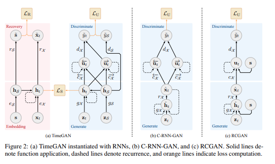
On the other hand, multiple studies have straightforwardly inherited the GAN framework within the temporal setting. The first (C-RNN-GAN) [4] directly applied the GAN architecture to sequential data, using LSTM networks for generator and discriminator. Data is generated recurrently, taking as inputs a noise vector and the data generated from the previous time step. Recurrent Conditional GAN (RCGAN) [5] took a similar approach, introducing minor architectural differences such as dropping the dependence on the previous output while conditioning on additional input [14]. A multitude of applied studies have since utilized these frameworks to generate synthetic sequences in such diverse domains as text [15], finance [16], biosignals [17], sensor [18] and smart grid data [19], as well as renewable scenarios [20]. Recent work [6] has proposed conditioning on time stamp information to handle irregularly sampling. However, unlike our proposed technique, these approaches rely only on the binary adversarial feedback for learning, which by itself may not be sufficient to guarantee specifically that the network efficiently captures the temporal dynamics in the training data.

中文翻译：

另一方面，许多研究直接继承了 GAN 框架用于时间序列场景。首个代表作 C-RNN-GAN [4] 直接将 GAN 架构应用于序列数据，使用 LSTM 网络作为生成器和判别器。数据是循环生成的，输入包括噪声向量和上一步生成的数据。循环条件 GAN (RCGAN) [5] 采用了类似的方法，引入了微小的架构差异，例如去除了对前一输出的依赖，同时以额外输入为条件 [14]。此后，许多应用研究利用这些框架在文本 [15]、金融 [16]、生物信号 [17]、传感器 [18]、智能电网数据 [19] 以及可再生能源场景 [20] 等多个领域生成合成序列。最近的工作 [6] 提出以时间戳信息为条件来处理不规则采样。然而，与我们要提出的技术不同，这些方法仅依赖于**二元对抗反馈（即真/假判别）**进行学习，这本身可能不足以保证网络能够有效地捕捉训练数据中的时间动态。

💡 解读：

这一段批判了现有的 Time-Series GANs：它们虽然引入了随机噪声（解决了"确定性"问题），但太过于依赖判别器（Discriminator）的"True/False"打分。对于复杂的时间序列，仅靠判别器告诉生成器"这不像真的"，很难教会生成器学会精细的"ttt 时刻到 t+1t+1t+1 时刻"的物理转换规律。

第四段：表示学习 (Representation Learning)

Finally, representation learning in the time-series setting primarily deals with the benefits of learning compact encodings for the benefit of downstream tasks such as prediction [21], forecasting [22], and classification [23]. Other works have studied the utility of learning latent representations for purposes of pre-training [24], disentanglement [25], and interpretability [26]. Meanwhile in the static setting, several works have explored the benefit of combining autoencoders with adversarial training, with objectives such as learning similarity measures [27], enabling efficient inference [28], as well as improving generative capability [29]---an approach that has subsequently been applied to generating discrete structures by encoding and generating entire sequences for discrimination [30]. By contrast, our proposed method generalizes to arbitrary time-series data, incorporates stochasticity at each time step, as well as employing an embedding network to identify a lower-dimensional space for the generative model to learn the stepwise distributions and latent dynamics of the data.

中文翻译：

最后，时间序列背景下的表示学习主要涉及学习紧凑编码的好处，以服务于预测 [21]、预报 [22] 和分类 [23] 等下游任务。其他工作研究了学习潜在表示在预训练 [24]、解纠缠 [25] 和可解释性 [26] 方面的效用。同时，在静态数据背景下，一些工作探索了将自动编码器（Autoencoders）与对抗训练相结合的好处，其目标包括学习相似性度量 [27]、实现高效推理 [28] 以及提高生成能力 [29]------这种方法随后被应用于通过编码和生成整个序列进行判别来生成离散结构 [30]。相比之下，我们要提出的方法推广到了任意时间序列数据，在每个时间步都引入了随机性，并采用了一个嵌入网络来识别一个低维空间，以便生成模型学习数据的逐步分布和潜在动态。

3 Problem Formulation (问题定义)

第一段：符号定义与数据结构

原文：

Consider the general data setting where each instance consists of two elements: static features (that do not change over time, e.g. gender), and temporal features (that occur over time, e.g. vital signs). Let S\mathcal{S}S be a vector space of static features, X\mathcal{X}X of temporal features, and let S∈S,X∈X\mathbf{S} \in \mathcal{S}, \mathbf{X} \in \mathcal{X}S∈S,X∈X be random vectors that can be instantiated with specific values denoted s\mathbf{s}s and x\mathbf{x}x. We consider tuples of the form (S,X1:T)(\mathbf{S}, \mathbf{X}{1:T})(S,X1:T) with some joint distribution ppp. The length TTT of each sequence is also a random variable, the distribution of which---for notational convenience---we absorb into ppp. In the training data, let individual samples be indexed by n∈{1,...,N}n \in \{1, ..., N\}n∈{1,...,N}, so we can denote the training dataset D={(sn,xn,1:Tn)}n=1N\mathcal{D} = \{(\mathbf{s}n, \mathbf{x}{n,1:T_n})\}{n=1}^ND={(sn,xn,1:Tn)}n=1N. Going forward, subscripts nnn are omitted unless explicitly required.

中文翻译：

考虑一个通用的数据设置，其中每个实例由两个元素组成：静态特征 （随时间不变，例如性别）和时序特征 （随时间发生，例如生命体征）。设 S\mathcal{S}S 为静态特征的向量空间，X\mathcal{X}X 为时序特征的向量空间，并设 S∈S,X∈X\mathbf{S} \in \mathcal{S}, \mathbf{X} \in \mathcal{X}S∈S,X∈X 为可以实例化为特定值 s\mathbf{s}s 和 x\mathbf{x}x 的随机向量。我们考虑形式为 (S,X1:T)(\mathbf{S}, \mathbf{X}{1:T})(S,X1:T) 的元组，其具有某种联合分布 ppp。每个序列的长度 TTT 也是一个随机变量，为了符号方便，我们将 TTT 的分布吸收到 ppp 中。在训练数据中，设样本索引为 n∈{1,...,N}n \in \{1, ..., N\}n∈{1,...,N}，因此我们可以表示训练数据集为 D={(sn,xn,1:Tn)}n=1N\mathcal{D} = \{(\mathbf{s}n, \mathbf{x}{n,1:T_n})\}{n=1}^ND={(sn,xn,1:Tn)}n=1N。在下文中，除非明确需要，否则将省略下标 nnn。

💡 专家解读：

这里 TimeGAN 做了一个比普通 RNN 更细致的区分：

S\mathbf{S}S (Static): 静态数据。比如在医疗数据中，病人的年龄、性别、基因型是不随时间变的。很多模型忽略了这一点，但这对于生成高质量数据很重要（例如：女性患者可能有不同的心率模式）。
X1:T\mathbf{X}_{1:T}X1:T (Temporal): 动态时序数据。比如连续 24 小时的血压监测值。

第二段：目标分解（联合分布 vs 条件分布）

原文：

Our goal is to use training data D\mathcal{D}D to learn a density p^(S,X1:T)\hat{p}(\mathbf{S}, \mathbf{X}{1:T})p^(S,X1:T) that best approximates p(S,X1:T)p(\mathbf{S}, \mathbf{X}{1:T})p(S,X1:T). This is a high-level objective, and---depending on the lengths, dimensionality, and distribution of the data---may be difficult to optimize in the standard GAN framework. Therefore we additionally make use of the autoregressive decomposition of the joint p(S,X1:T)=p(S)∏tp(Xt∣S,X1:t−1)p(\mathbf{S}, \mathbf{X}_{1:T}) = p(\mathbf{S}) \prod_t p(\mathbf{X}t|\mathbf{S}, \mathbf{X}{1:t-1})p(S,X1:T)=p(S)∏tp(Xt∣S,X1:t−1) to focus specifically on the conditionals, yielding the complementary---and simpler---objective of learning a density p^(Xt∣S,X1:t−1)\hat{p}(\mathbf{X}t|\mathbf{S}, \mathbf{X}{1:t-1})p^(Xt∣S,X1:t−1) that best approximates p(Xt∣S,X1:t−1)p(\mathbf{X}t|\mathbf{S}, \mathbf{X}{1:t-1})p(Xt∣S,X1:t−1) at any time ttt.

中文翻译：

我们的目标是使用训练数据 D\mathcal{D}D 学习一个密度函数 p^(S,X1:T)\hat{p}(\mathbf{S}, \mathbf{X}{1:T})p^(S,X1:T)，使其最好地逼近真实分布 p(S,X1:T)p(\mathbf{S}, \mathbf{X}{1:T})p(S,X1:T)。这是一个高层次的目标，并且------取决于数据的长度、维度和分布------在标准 GAN 框架中可能难以优化。因此，我们额外利用了联合分布的自回归分解 p(S,X1:T)=p(S)∏tp(Xt∣S,X1:t−1)p(\mathbf{S}, \mathbf{X}_{1:T}) = p(\mathbf{S}) \prod_t p(\mathbf{X}t|\mathbf{S}, \mathbf{X}{1:t-1})p(S,X1:T)=p(S)∏tp(Xt∣S,X1:t−1)，以专门关注条件概率，从而产生了一个互补且更简单的目标：学习一个密度 p^(Xt∣S,X1:t−1)\hat{p}(\mathbf{X}t|\mathbf{S}, \mathbf{X}{1:t-1})p^(Xt∣S,X1:t−1)，使其在任何时间 ttt 都最好地逼近 p(Xt∣S,X1:t−1)p(\mathbf{X}t|\mathbf{S}, \mathbf{X}{1:t-1})p(Xt∣S,X1:t−1)。

💡 解读：

这是 TimeGAN 理论的核心。作者认为直接学整个大序列的分布 p(S,X1:T)p(\mathbf{S}, \mathbf{X}_{1:T})p(S,X1:T) 太难了（维度高、太复杂）。但是，如果我们把它拆解（Decomposition）：
整个序列概率=静态特征概率×∏(基于过去预测现在的概率) \text{整个序列概率} = \text{静态特征概率} \times \prod (\text{基于过去预测现在的概率}) 整个序列概率=静态特征概率×∏(基于过去预测现在的概率)

即：先生成性别，再基于性别和前一秒心率生成下一秒心率。这样就把一个生成问题 部分转化为了一个预测问题。

第三段：两个目标函数 (Global vs Local)

原文：

Two Objectives. Importantly, this breaks down the sequence-level objective (matching the joint distribution) into a series of stepwise objectives (matching the conditionals). The first is global,
min⁡p^D(p(S,X1:T)∥p^(S,X1:T))(1) \min_{\hat{p}} D(p(\mathbf{S}, \mathbf{X}{1:T}) \| \hat{p}(\mathbf{S}, \mathbf{X}{1:T})) \quad \quad (1) p^minD(p(S,X1:T)∥p^(S,X1:T))(1)

where DDD is some appropriate measure of distance between distributions. The second is local,
min⁡p^D(p(Xt∣S,X1:t−1)∥p^(Xt∣S,X1:t−1))(2) \min_{\hat{p}} D(p(\mathbf{X}t|\mathbf{S}, \mathbf{X}{1:t-1}) \| \hat{p}(\mathbf{X}t|\mathbf{S}, \mathbf{X}{1:t-1})) \quad \quad (2) p^minD(p(Xt∣S,X1:t−1)∥p^(Xt∣S,X1:t−1))(2)

for any ttt. Under an ideal discriminator in the GAN framework, the former takes the form of the Jensen-Shannon divergence. Using the original data for supervision via maximum-likelihood (ML) training, the latter takes the form of the Kullback-Leibler divergence. Note that minimizing the former relies on the presence of a perfect adversary (which we may not have access to), while minimizing the latter only depends on the presence of ground-truth sequences (which we do have access to). Our target, then, will be a combination of the GAN objective (proportional to Expression 1) and the ML objective (proportional to Expression 2). As we shall see, this naturally yields a training procedure that involves the simple addition of a supervised loss to guide adversarial learning.

中文翻译：
两个目标。 重要的是，这将序列级目标（匹配联合分布）分解为一系列逐步目标（匹配条件分布）。

第一个是全局目标 ：
min⁡p^D(p(S,X1:T)∥p^(S,X1:T))(1) \min_{\hat{p}} D(p(\mathbf{S}, \mathbf{X}{1:T}) \| \hat{p}(\mathbf{S}, \mathbf{X}{1:T})) \quad \quad (1) p^minD(p(S,X1:T)∥p^(S,X1:T))(1)

其中 DDD 是某种适当的分布间距离度量。

第二个是局部目标 ：
min⁡p^D(p(Xt∣S,X1:t−1)∥p^(Xt∣S,X1:t−1))(2) \min_{\hat{p}} D(p(\mathbf{X}t|\mathbf{S}, \mathbf{X}{1:t-1}) \| \hat{p}(\mathbf{X}t|\mathbf{S}, \mathbf{X}{1:t-1})) \quad \quad (2) p^minD(p(Xt∣S,X1:t−1)∥p^(Xt∣S,X1:t−1))(2)

对于任意 ttt。在 GAN 框架下的理想判别器中，前者（公式 1）采用 Jensen-Shannon 散度 的形式。通过最大似然（ML）训练使用原始数据进行监督，后者（公式 2）采用 Kullback-Leibler 散度的形式。请注意，最小化前者依赖于存在一个完美的对抗者（我们可能无法获得），而最小化后者仅取决于存在真实序列（我们可以获得）。因此，我们的目标将是 GAN 目标（与表达式 1 成正比）和 ML 目标（与表达式 2 成正比）的结合。正如我们将看到的，这自然产生了一个训练过程，即简单地添加一个**监督损失（Supervised Loss）**来指导对抗学习。

💡 解读：

这里作者用严谨的数学语言解释了为什么要"混搭"损失函数：

公式 (1) 全局目标 : 就是标准的 GAN Loss。它希望生成的整个序列看起来像真的。这对应于 Unsupervised Loss (LUL_ULU)。
公式 (2) 局部目标 : 就是标准的回归/预测 Loss。它希望模型能学会"下一步会发生什么"。这对应于 Supervised Loss (LSL_SLS)。

结论：
TimeGAN Loss≈GAN Loss (像不像)+Supervised Loss (准不准) \text{TimeGAN Loss} \approx \text{GAN Loss (像不像)} + \text{Supervised Loss (准不准)} TimeGAN Loss≈GAN Loss (像不像)+Supervised Loss (准不准)

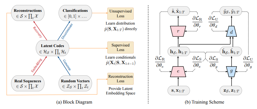
4 Proposed Model: Time-series GAN (TimeGAN)

原文（引言部分）:

TimeGAN consists of four network components: an embedding function, recovery function, sequence generator, and sequence discriminator. The key insight is that the autoencoding components (first two) are trained jointly with the adversarial components (latter two), such that TimeGAN simultaneously learns to encode features, generate representations, and iterate across time. The embedding network provides the latent space, the adversarial network operates within this space, and the latent dynamics of both real and synthetic data are synchronized through a supervised loss. We describe each in turn.

中文翻译（引言部分）:

TimeGAN 由四个网络组件构成：一个嵌入函数、一个恢复函数、一个序列生成器和一个序列判别器。其关键思想在于，自动编码组件（前两个）与对抗组件（后两个）是联合训练的，从而使得 TimeGAN 能够同时学习编码特征、生成表示以及在时间上进行迭代。嵌入网络提供了潜在空间，对抗网络在这个空间内运作，而真实数据和合成数据的潜在动态则通过一个有监督损失进行同步。我们依次对每个组件进行描述。

4.1 Embedding and Recovery Functions

原文:

The embedding and recovery functions provide mappings between feature and latent space, allowing the adversarial network to learn the underlying temporal dynamics of the data via lower-dimensional representations. Let HS,HX\mathcal{H}{\mathcal{S}}, \mathcal{H}{\mathcal{X}}HS,HX denote the latent vector spaces corresponding to feature spaces S,X\mathcal{S}, \mathcal{X}S,X. Then the embedding function e:S×∏tX→HS×∏tHXe : \mathcal{S} \times \prod_t \mathcal{X} \rightarrow \mathcal{H}{\mathcal{S}} \times \prod_t \mathcal{H}{\mathcal{X}}e:S×∏tX→HS×∏tHX takes static and temporal features to their latent codes hS,h1:T=e(s,x1:T)\mathbf{h}{\mathcal{S}}, \mathbf{h}{1:T} = e(\mathbf{s}, \mathbf{x}{1:T})hS,h1:T=e(s,x1:T). In this paper, we implement eee via a recurrent network,
hS=eS(s),ht=eX(hS,ht−1,xt)(3) \mathbf{h}{\mathcal{S}} = e_{\mathcal{S}}(\mathbf{s}), \quad \mathbf{h}t = e{\mathcal{X}}(\mathbf{h}{\mathcal{S}}, \mathbf{h}{t-1}, \mathbf{x}_t) \quad (3) hS=eS(s),ht=eX(hS,ht−1,xt)(3)

where eS:S→HSe_{\mathcal{S}} : \mathcal{S} \rightarrow \mathcal{H}{\mathcal{S}}eS:S→HS is an embedding network for static features, and eX:HS×HX×X→HXe{\mathcal{X}} : \mathcal{H}{\mathcal{S}} \times \mathcal{H}{\mathcal{X}} \times \mathcal{X} \rightarrow \mathcal{H}{\mathcal{X}}eX:HS×HX×X→HX a recurrent embedding network for temporal features. In the opposite direction, the recovery function r:HS×∏tHX→S×∏tXr : \mathcal{H}{\mathcal{S}} \times \prod_t \mathcal{H}{\mathcal{X}} \rightarrow \mathcal{S} \times \prod_t \mathcal{X}r:HS×∏tHX→S×∏tX takes static and temporal codes back to their feature representations s~,x~1:T=r(hS,h1:T)\tilde{\mathbf{s}}, \tilde{\mathbf{x}}{1:T} = r(\mathbf{h}{\mathcal{S}}, \mathbf{h}{1:T})s~,x~1:T=r(hS,h1:T). Here we implement rrr through a feedforward network at each step,
s~=rS(hS),x~t=rX(ht)(4) \tilde{\mathbf{s}} = r_{\mathcal{S}}(\mathbf{h}_{\mathcal{S}}), \quad \tilde{\mathbf{x}}t = r{\mathcal{X}}(\mathbf{h}_t) \quad (4) s~=rS(hS),x~t=rX(ht)(4)

where rS:HS→Sr_{\mathcal{S}} : \mathcal{H}{\mathcal{S}} \rightarrow \mathcal{S}rS:HS→S and rX:HX→Xr{\mathcal{X}} : \mathcal{H}_{\mathcal{X}} \rightarrow \mathcal{X}rX:HX→X are recovery networks for static and temporal embeddings. Note that the embedding and recovery functions can be parameterized by any architecture of choice, with the only stipulation being that they be autoregressive and obey causal ordering (i.e. output(s) at each step can only depend on preceding information). For example, it is just as possible to implement the former with temporal convolutions, or the latter via an attention-based decoder. Here we choose implementations 3 and 4 as a minimal example to isolate the source of gains.

中文翻译:

嵌入和恢复函数提供了特征空间与潜在空间之间的映射，允许对抗网络通过低维表示学习数据的潜在时间动态。设 HS,HX\mathcal{H}{\mathcal{S}}, \mathcal{H}{\mathcal{X}}HS,HX 表示对应于特征空间 S,X\mathcal{S}, \mathcal{X}S,X 的潜在向量空间。嵌入函数 e:S×∏tX→HS×∏tHXe : \mathcal{S} \times \prod_t \mathcal{X} \rightarrow \mathcal{H}{\mathcal{S}} \times \prod_t \mathcal{H}{\mathcal{X}}e:S×∏tX→HS×∏tHX 将静态和时序特征转换为它们的潜在编码 hS,h1:T=e(s,x1:T)\mathbf{h}{\mathcal{S}}, \mathbf{h}{1:T} = e(\mathbf{s}, \mathbf{x}{1:T})hS,h1:T=e(s,x1:T)。在本文中，我们通过一个循环网络来实现 eee，
hS=eS(s),ht=eX(hS,ht−1,xt)(3) \mathbf{h}{\mathcal{S}} = e_{\mathcal{S}}(\mathbf{s}), \quad \mathbf{h}t = e{\mathcal{X}}(\mathbf{h}{\mathcal{S}}, \mathbf{h}{t-1}, \mathbf{x}_t) \quad (3) hS=eS(s),ht=eX(hS,ht−1,xt)(3)

其中 eS:S→HSe_{\mathcal{S}} : \mathcal{S} \rightarrow \mathcal{H}{\mathcal{S}}eS:S→HS 是用于静态特征的嵌入网络，而 eX:HS×HX×X→HXe{\mathcal{X}} : \mathcal{H}{\mathcal{S}} \times \mathcal{H}{\mathcal{X}} \times \mathcal{X} \rightarrow \mathcal{H}_{\mathcal{X}}eX:HS×HX×X→HX 是用于时序特征的循环嵌入网络。

在相反方向，恢复函数 r:HS×∏tHX→S×∏tXr : \mathcal{H}{\mathcal{S}} \times \prod_t \mathcal{H}{\mathcal{X}} \rightarrow \mathcal{S} \times \prod_t \mathcal{X}r:HS×∏tHX→S×∏tX 将静态和时序编码还原回它们的特征表示 s~,x~1:T=r(hS,h1:T)\tilde{\mathbf{s}}, \tilde{\mathbf{x}}{1:T} = r(\mathbf{h}{\mathcal{S}}, \mathbf{h}{1:T})s~,x~1:T=r(hS,h1:T)。这里我们在每一步通过一个前馈网络来实现 rrr，
s~=rS(hS),x~t=rX(ht)(4) \tilde{\mathbf{s}} = r{\mathcal{S}}(\mathbf{h}_{\mathcal{S}}), \quad \tilde{\mathbf{x}}t = r{\mathcal{X}}(\mathbf{h}_t) \quad (4) s~=rS(hS),x~t=rX(ht)(4)

其中 rS:HS→Sr_{\mathcal{S}} : \mathcal{H}{\mathcal{S}} \rightarrow \mathcal{S}rS:HS→S 和 rX:HX→Xr{\mathcal{X}} : \mathcal{H}_{\mathcal{X}} \rightarrow \mathcal{X}rX:HX→X 分别是用于静态和时序嵌入的恢复网络。

请注意，嵌入和恢复函数可以由任何选择的架构进行参数化，唯一的规定是它们必须是自回归的并遵守因果顺序（即，每一步的输出只能依赖于之前的信息）。例如，同样可以用时间卷积实现前者，或用基于注意力的解码器实现后者。这里我们选择实现方式 3 和 4 作为一个最小化的例子，以分离出增益的来源。

4.2 Sequence Generator and Discriminator

原文:

Instead of producing synthetic output directly in feature space, the generator first outputs into the embedding space. Let ZS,ZX\mathcal{Z}{\mathcal{S}}, \mathcal{Z}{\mathcal{X}}ZS,ZX denote vector spaces over which known distributions are defined, and from which random vectors are drawn as input for generating into HS,HX\mathcal{H}{\mathcal{S}}, \mathcal{H}{\mathcal{X}}HS,HX. Then the generating function g:ZS×∏tZX→HS×∏tHXg : \mathcal{Z}{\mathcal{S}} \times \prod_t \mathcal{Z}{\mathcal{X}} \rightarrow \mathcal{H}{\mathcal{S}} \times \prod_t \mathcal{H}{\mathcal{X}}g:ZS×∏tZX→HS×∏tHX takes a tuple of static and temporal random vectors to synthetic latent codes h^S,h^1:T=g(zS,z1:T)\hat{\mathbf{h}}{\mathcal{S}}, \hat{\mathbf{h}}{1:T} = g(\mathbf{z}{\mathcal{S}}, \mathbf{z}{1:T})h^S,h^1:T=g(zS,z1:T). We implement ggg through a recurrent network,
h^S=gS(zS),h^t=gX(h^S,h^t−1,zt)(5) \hat{\mathbf{h}}{\mathcal{S}} = g{\mathcal{S}}(\mathbf{z}{\mathcal{S}}), \quad \hat{\mathbf{h}}t = g{\mathcal{X}}(\hat{\mathbf{h}}{\mathcal{S}}, \hat{\mathbf{h}}_{t-1}, \mathbf{z}_t) \quad (5) h^S=gS(zS),h^t=gX(h^S,h^t−1,zt)(5)

where gS:ZS→HSg_{\mathcal{S}} : \mathcal{Z}{\mathcal{S}} \rightarrow \mathcal{H}{\mathcal{S}}gS:ZS→HS is a generator network for static features, and gX:HS×HX×ZX→HXg_{\mathcal{X}} : \mathcal{H}{\mathcal{S}} \times \mathcal{H}{\mathcal{X}} \times \mathcal{Z}{\mathcal{X}} \rightarrow \mathcal{H}{\mathcal{X}}gX:HS×HX×ZX→HX is a recurrent generator for temporal features. Random vector zS\mathbf{z}{\mathcal{S}}zS can be sampled from a distribution of choice, and zt\mathbf{z}tzt follows a stochastic process; here we use the Gaussian distribution and Wiener process respectively. Finally, the discriminator also operates from the embedding space. The discrimination function d:HS×∏tHX→×∏td : \mathcal{H}{\mathcal{S}} \times \prod_t \mathcal{H}{\mathcal{X}} \rightarrow \times \prod_td:HS×∏tHX→×∏t receives the static and temporal codes, returning classifications y~S,y~1:T=d(h~S,h~1:T)\tilde{y}{\mathcal{S}}, \tilde{y}{1:T} = d(\tilde{\mathbf{h}}{\mathcal{S}}, \tilde{\mathbf{h}}{1:T})y~S,y~1:T=d(h~S,h~1:T). The h∗\mathbf{h}*h∗ notation denotes either real (h∗\mathbf{h}*h∗) or synthetic (h^∗\hat{\mathbf{h}}*h^∗) embeddings; similarly, the y~\tilde{y}y~ notation denotes classifications of either real (y∗\mathbf{y}*y∗) or synthetic (y^∗\hat{\mathbf{y}}*y^∗) data. Here we implement ddd via a bidirectional recurrent network with a feedforward output layer,
y~S=dS(hS)y~t=dX(u→t,u←t)(6) \tilde{y}{\mathcal{S}} = d_{\mathcal{S}}(\mathbf{h}_{\mathcal{S}}) \quad \tilde{y}t = d{\mathcal{X}}(\overrightarrow{\mathbf{u}}_t, \overleftarrow{\mathbf{u}}_t) \quad (6) y~S=dS(hS)y~t=dX(u t,u t)(6)

where u→t=c→X(hS,ht,u→t−1)\overrightarrow{\mathbf{u}}t = \overrightarrow{c}{\mathcal{X}}(\mathbf{h}{\mathcal{S}}, \mathbf{h}t, \overrightarrow{\mathbf{u}}{t-1})u t=c X(hS,ht,u t−1) and u←t=c←X(hS,ht,u←t+1)\overleftarrow{\mathbf{u}}t = \overleftarrow{c}{\mathcal{X}}(\mathbf{h}{\mathcal{S}}, \mathbf{h}t, \overleftarrow{\mathbf{u}}{t+1})u t=c X(hS,ht,u t+1) respectively denote the sequences of forward and backward hidden states, c→X,c←X\overrightarrow{c}{\mathcal{X}}, \overleftarrow{c}{\mathcal{X}}c X,c X are recurrent functions, and dS,dXd_{\mathcal{S}}, d_{\mathcal{X}}dS,dX are output layer classification functions. Similarly, there are no restrictions on architecture beyond the generator being autoregressive; here we use a standard recurrent formulation for ease of exposition.

中文翻译:

生成器不直接在特征空间产生合成输出，而是首先输出到嵌入空间。设 ZS,ZX\mathcal{Z}{\mathcal{S}}, \mathcal{Z}{\mathcal{X}}ZS,ZX 为定义了已知分布的向量空间，并从中抽取随机向量作为生成到 HS,HX\mathcal{H}{\mathcal{S}}, \mathcal{H}{\mathcal{X}}HS,HX 的输入。生成函数 g:ZS×∏tZX→HS×∏tHXg : \mathcal{Z}{\mathcal{S}} \times \prod_t \mathcal{Z}{\mathcal{X}} \rightarrow \mathcal{H}{\mathcal{S}} \times \prod_t \mathcal{H}{\mathcal{X}}g:ZS×∏tZX→HS×∏tHX 接收一个静态和时序随机向量的元组，并将其转换为合成的潜在编码 h^S,h^1:T=g(zS,z1:T)\hat{\mathbf{h}}{\mathcal{S}}, \hat{\mathbf{h}}{1:T} = g(\mathbf{z}{\mathcal{S}}, \mathbf{z}{1:T})h^S,h^1:T=g(zS,z1:T)。我们通过一个循环网络来实现 ggg，
h^S=gS(zS),h^t=gX(h^S,h^t−1,zt)(5) \hat{\mathbf{h}}{\mathcal{S}} = g{\mathcal{S}}(\mathbf{z}{\mathcal{S}}), \quad \hat{\mathbf{h}}t = g{\mathcal{X}}(\hat{\mathbf{h}}{\mathcal{S}}, \hat{\mathbf{h}}_{t-1}, \mathbf{z}_t) \quad (5) h^S=gS(zS),h^t=gX(h^S,h^t−1,zt)(5)

其中 gS:ZS→HSg_{\mathcal{S}} : \mathcal{Z}{\mathcal{S}} \rightarrow \mathcal{H}{\mathcal{S}}gS:ZS→HS 是用于静态特征的生成器网络，而 gX:HS×HX×ZX→HXg_{\mathcal{X}} : \mathcal{H}{\mathcal{S}} \times \mathcal{H}{\mathcal{X}} \times \mathcal{Z}{\mathcal{X}} \rightarrow \mathcal{H}{\mathcal{X}}gX:HS×HX×ZX→HX 是用于时序特征的循环生成器。随机向量 zS\mathbf{z}_{\mathcal{S}}zS 可以从任意选择的分布中采样，而 zt\mathbf{z}_tzt 则遵循一个随机过程；这里我们分别使用高斯分布和维纳过程。

最后，判别器也在嵌入空间中运作。判别函数 d:HS×∏tHX→×∏td : \mathcal{H}{\mathcal{S}} \times \prod_t \mathcal{H}{\mathcal{X}} \rightarrow \times \prod_td:HS×∏tHX→×∏t 接收静态和时序编码，返回分类结果 y~S,y~1:T=d(h~S,h~1:T)\tilde{y}{\mathcal{S}}, \tilde{y}{1:T} = d(\tilde{\mathbf{h}}{\mathcal{S}}, \tilde{\mathbf{h}}{1:T})y~S,y~1:T=d(h~S,h~1:T)。符号 h∗\mathbf{h}*h∗ 表示真实的 (h∗\mathbf{h}*h∗) 或合成的 (h^∗\hat{\mathbf{h}}*h^∗) 嵌入；类似地，符号 y~\tilde{y}y~ 表示对真实 (y∗\mathbf{y}*y∗) 或合成 (y^∗\hat{\mathbf{y}}*y^∗) 数据的分类。这里我们通过一个带前馈输出层的双向循环网络来实现 ddd，
y~S=dS(hS)y~t=dX(u→t,u←t)(6) \tilde{y}{\mathcal{S}} = d_{\mathcal{S}}(\mathbf{h}_{\mathcal{S}}) \quad \tilde{y}t = d{\mathcal{X}}(\overrightarrow{\mathbf{u}}_t, \overleftarrow{\mathbf{u}}_t) \quad (6) y~S=dS(hS)y~t=dX(u t,u t)(6)

其中 u→t=c→X(hS,ht,u→t−1)\overrightarrow{\mathbf{u}}t = \overrightarrow{c}{\mathcal{X}}(\mathbf{h}{\mathcal{S}}, \mathbf{h}t, \overrightarrow{\mathbf{u}}{t-1})u t=c X(hS,ht,u t−1) 和 u←t=c←X(hS,ht,u←t+1)\overleftarrow{\mathbf{u}}t = \overleftarrow{c}{\mathcal{X}}(\mathbf{h}{\mathcal{S}}, \mathbf{h}t, \overleftarrow{\mathbf{u}}{t+1})u t=c X(hS,ht,u t+1) 分别表示前向和后向隐藏状态的序列，c→X,c←X\overrightarrow{c}{\mathcal{X}}, \overleftarrow{c}{\mathcal{X}}c X,c X 是循环函数，而 dS,dXd_{\mathcal{S}}, d_{\mathcal{X}}dS,dX 是输出层的分类函数。类似地，除了生成器必须是自回归的之外，对架构没有其他限制；这里为了便于阐述，我们使用了一个标准的循环公式。

4.3 Jointly Learning to Encode, Generate, and Iterate

原文:

First, purely as a reversible mapping between feature and latent spaces, the embedding and recovery functions should enable accurate reconstructions s~,x~1:T\tilde{\mathbf{s}}, \tilde{\mathbf{x}}{1:T}s~,x~1:T of the original data s,x1:T\mathbf{s}, \mathbf{x}{1:T}s,x1:T from their latent representations hS,h1:T\mathbf{h}{\mathcal{S}}, \mathbf{h}{1:T}hS,h1:T. Therefore our first objective function is the reconstruction loss ,
LR=Es,x1:T∼p[∣∣s−s~∣∣2+∑t∣∣xt−x~t∣∣2](7) \mathcal{L}R = \mathbb{E}{\mathbf{s}, \mathbf{x}_{1:T} \sim p} \left[ ||\mathbf{s} - \tilde{\mathbf{s}}||_2 + \sum_t ||\mathbf{x}_t - \tilde{\mathbf{x}}_t||_2 \right] \quad (7) LR=Es,x1:T∼p[∣∣s−s~∣∣2+t∑∣∣xt−x~t∣∣2](7)

In TimeGAN, the generator is exposed to two types of inputs during training. First, in pure open-loop mode, the generator---which is autoregressive---receives synthetic embeddings h^S,h^1:t−1\hat{\mathbf{h}}{\mathcal{S}}, \hat{\mathbf{h}}{1:t-1}h^S,h^1:t−1 (i.e. its own previous outputs) in order to generate the next synthetic vector h^t\hat{\mathbf{h}}th^t. Gradients are then computed on the unsupervised loss . This is as one would expect---that is, to allow maximizing (for the discriminator) or minimizing (for the generator) the likelihood of providing correct classifications y~S,y~1:T\tilde{y}{\mathcal{S}}, \tilde{y}{1:T}y~S,y~1:T for both the training data hS,h1:T\mathbf{h}{\mathcal{S}}, \mathbf{h}{1:T}hS,h1:T as well as for synthetic output h^S,h^1:T\hat{\mathbf{h}}{\mathcal{S}}, \hat{\mathbf{h}}{1:T}h^S,h^1:T from the generator,
LU=Es,x1:T∼p[log⁡yS+∑tlog⁡yt]+Es,x1:T∼p^[log⁡(1−y^S)+∑tlog⁡(1−y^t)](8) \mathcal{L}U = \mathbb{E}{\mathbf{s}, \mathbf{x}{1:T} \sim p} [\log y_S + \sum_t \log y_t] + \mathbb{E}{\mathbf{s}, \mathbf{x}{1:T} \sim \hat{p}} [\log(1 - \hat{y}_S) + \sum_t \log(1 - \hat{y}_t)] \quad (8) LU=Es,x1:T∼p[logyS+t∑logyt]+Es,x1:T∼p^[log(1−y^S)+t∑log(1−y^t)](8)

Relying solely on the discriminator's binary adversarial feedback may not be sufficient incentive for the generator to capture the stepwise conditional distributions in the data. To achieve this more efficiently, we introduce an additional loss to further discipline learning. In an alternating fashion, we also train in closed-loop mode, where the generator receives sequences of embeddings of actual data h1:t−1\mathbf{h}{1:t-1}h1:t−1 (i.e. computed by the embedding network) to generate the next latent vector. Gradients can now be computed on a loss that captures the discrepancy between distributions p(Ht∣HS,H1:t−1)p(\mathbf{H}t|\mathbf{H}{\mathcal{S}}, \mathbf{H}{1:t-1})p(Ht∣HS,H1:t−1) and p^(Ht∣HS,H1:t−1)\hat{p}(\mathbf{H}t|\mathbf{H}{\mathcal{S}}, \mathbf{H}{1:t-1})p^(Ht∣HS,H1:t−1). Applying maximum likelihood yields the familiar supervised loss ,
LS=Es,x1:T∼p[∑t∣∣ht−gX(hS,ht−1,zt)∣∣2](9) \mathcal{L}S = \mathbb{E}{\mathbf{s}, \mathbf{x}{1:T} \sim p} \left[ \sum_t ||\mathbf{h}t - g{\mathcal{X}}(\mathbf{h}{\mathcal{S}}, \mathbf{h}{t-1}, \mathbf{z}_t)||_2 \right] \quad (9) LS=Es,x1:T∼p[t∑∣∣ht−gX(hS,ht−1,zt)∣∣2](9)

where gX(hS,ht−1,zt)g_{\mathcal{X}}(\mathbf{h}{\mathcal{S}}, \mathbf{h}{t-1}, \mathbf{z}t)gX(hS,ht−1,zt) approximates Ezt∼N[p^(Ht∣HS,H1:t−1,zt)]\mathbb{E}{\mathbf{z}t \sim \mathcal{N}} [\hat{p}(\mathbf{H}t|\mathbf{H}{\mathcal{S}}, \mathbf{H}{1:t-1}, \mathbf{z}_t)]Ezt∼N[p^(Ht∣HS,H1:t−1,zt)] with one sample zt\mathbf{z}_tzt as is standard in stochastic gradient descent. In sum, at any step in a training sequence, we assess the difference between the actual next-step latent vector (from the embedding function) and synthetic next-step latent vector (from the generator---conditioned on the actual historical sequence of latents). While LU\mathcal{L}_ULU pushes the generator to create realistic sequences (evaluated by an imperfect adversary), LS\mathcal{L}SLS further ensures that it produces similar stepwise transitions (evaluated by ground-truth targets).
Optimization. Figure 1(b) illustrates the mechanics of our approach at training. Let θe,θr,θg,θd\theta_e, \theta_r, \theta_g, \theta_dθe,θr,θg,θd respectively denote the parameters of the embedding, recovery, generator, and discriminator networks. The first two components are trained on both the reconstruction and supervised losses,
min⁡θe,θr(λLS+LR)(10) \min{\theta_e, \theta_r} (\lambda \mathcal{L}_S + \mathcal{L}_R) \quad (10) θe,θrmin(λLS+LR)(10)

where λ≥0\lambda \geq 0λ≥0 is a hyperparameter that balances the two losses. Importantly, LS\mathcal{L}_SLS is included such that the embedding process not only serves to reduce the dimensions of the adversarial learning space---it is actively conditioned to facilitate the generator in learning temporal relationships from the data.

Next, the generator and discriminator networks are trained adversarially as follows,
min⁡θg(ηLS+max⁡θdLU)(11) \min_{\theta_g} (\eta \mathcal{L}S + \max{\theta_d} \mathcal{L}_U) \quad (11) θgmin(ηLS+θdmaxLU)(11)

where η≥0\eta \geq 0η≥0 is another hyperparameter that balances the two losses. That is, in addition to the unsupervised minimax game played over classification accuracy, the generator additionally minimizes the supervised loss. By combining the objectives in this manner, TimeGAN is simultaneously trained to encode (feature vectors), generate (latent representations), and iterate (across time).

In practice, we find that TimeGAN is not sensitive to λ\lambdaλ and η\etaη; for all experiments in Section 5, we set λ=1\lambda = 1λ=1 and η=10\eta = 10η=10. Note that while GANs in general are not known for their ease of training, we do not discover any additional complications in TimeGAN. The embedding task serves to regularize adversarial learning---which now occurs in a lower-dimensional latent space. Similarly, the supervised loss has a constraining effect on the stepwise dynamics of the generator. For both reasons, we do not expect TimeGAN to be more challenging to train, and standard techniques for improving GAN training are still applicable. Algorithm pseudocode and illustrations with additional detail can be found in the Supplementary Materials.

中文翻译:

首先，纯粹作为特征空间和潜在空间之间的可逆映射，嵌入和恢复函数应当能够从潜在表示 hS,h1:T\mathbf{h}{\mathcal{S}}, \mathbf{h}{1:T}hS,h1:T 中准确重建出原始数据 s,x1:T\mathbf{s}, \mathbf{x}{1:T}s,x1:T 的重建值 s~,x~1:T\tilde{\mathbf{s}}, \tilde{\mathbf{x}}{1:T}s~,x~1:T。因此，我们的第一个目标函数是重建损失 ，
LR=Es,x1:T∼p[∣∣s−s~∣∣2+∑t∣∣xt−x~t∣∣2](7) \mathcal{L}R = \mathbb{E}{\mathbf{s}, \mathbf{x}_{1:T} \sim p} \left[ ||\mathbf{s} - \tilde{\mathbf{s}}||_2 + \sum_t ||\mathbf{x}_t - \tilde{\mathbf{x}}_t||_2 \right] \quad (7) LR=Es,x1:T∼p[∣∣s−s~∣∣2+t∑∣∣xt−x~t∣∣2](7)

在 TimeGAN 中，生成器在训练期间接触两种类型的输入。首先，在纯开环（open-loop）模式下，生成器------它是自回归的------接收合成的嵌入 h^S,h^1:t−1\hat{\mathbf{h}}{\mathcal{S}}, \hat{\mathbf{h}}{1:t-1}h^S,h^1:t−1（即它自己先前的输出），以生成下一个合成向量 h^t\hat{\mathbf{h}}_th^t。然后基于无监督损失计算梯度。这正如预期的那样------即允许最大化（对于判别器）或最小化（对于生成器）为训练数据 hS,h1:T\mathbf{h}{\mathcal{S}}, \mathbf{h}{1:T}hS,h1:T 以及生成器输出的合成数据 h^S,h^1:T\hat{\mathbf{h}}{\mathcal{S}}, \hat{\mathbf{h}}{1:T}h^S,h^1:T 提供正确分类 y~S,y~1:T\tilde{y}{\mathcal{S}}, \tilde{y}{1:T}y~S,y~1:T 的似然，
LU=Es,x1:T∼p[log⁡yS+∑tlog⁡yt]+Es,x1:T∼p^[log⁡(1−y^S)+∑tlog⁡(1−y^t)](8) \mathcal{L}U = \mathbb{E}{\mathbf{s}, \mathbf{x}{1:T} \sim p} [\log y_S + \sum_t \log y_t] + \mathbb{E}{\mathbf{s}, \mathbf{x}_{1:T} \sim \hat{p}} [\log(1 - \hat{y}_S) + \sum_t \log(1 - \hat{y}_t)] \quad (8) LU=Es,x1:T∼p[logyS+t∑logyt]+Es,x1:T∼p^[log(1−y^S)+t∑log(1−y^t)](8)

仅依赖判别器的二元对抗反馈可能不足以激励生成器捕捉数据中的逐步条件分布。为了更有效地实现这一点，我们引入了一个额外的损失来进一步约束学习。我们以交替方式在闭环（closed-loop）模式下训练，其中生成器接收真实数据 的嵌入序列 h1:t−1\mathbf{h}{1:t-1}h1:t−1（即由嵌入网络计算得出）来生成下一个潜在向量。现在的梯度可以基于一个损失来计算，该损失捕捉分布 p(Ht∣HS,H1:t−1)p(\mathbf{H}t|\mathbf{H}{\mathcal{S}}, \mathbf{H}{1:t-1})p(Ht∣HS,H1:t−1) 和 p^(Ht∣HS,H1:t−1)\hat{p}(\mathbf{H}t|\mathbf{H}{\mathcal{S}}, \mathbf{H}{1:t-1})p^(Ht∣HS,H1:t−1) 之间的差异。应用最大似然法产生了熟悉的有监督损失 ，
LS=Es,x1:T∼p[∑t∣∣ht−gX(hS,ht−1,zt)∣∣2](9) \mathcal{L}S = \mathbb{E}{\mathbf{s}, \mathbf{x}{1:T} \sim p} \left[ \sum_t ||\mathbf{h}t - g{\mathcal{X}}(\mathbf{h}{\mathcal{S}}, \mathbf{h}{t-1}, \mathbf{z}_t)||_2 \right] \quad (9) LS=Es,x1:T∼p[t∑∣∣ht−gX(hS,ht−1,zt)∣∣2](9)

其中 gX(hS,ht−1,zt)g_{\mathcal{X}}(\mathbf{h}{\mathcal{S}}, \mathbf{h}{t-1}, \mathbf{z}_t)gX(hS,ht−1,zt) 用一个样本 zt\mathbf{z}tzt 来近似 Ezt∼N[p^(Ht∣HS,H1:t−1,zt)]\mathbb{E}{\mathbf{z}t \sim \mathcal{N}} [\hat{p}(\mathbf{H}t|\mathbf{H}{\mathcal{S}}, \mathbf{H}{1:t-1}, \mathbf{z}_t)]Ezt∼N[p^(Ht∣HS,H1:t−1,zt)]，这在随机梯度下降中是标准做法。总之，在训练序列的任何一步，我们评估了实际的下一步潜在向量（来自嵌入函数）与合成的下一步潜在向量（来自生成器------以真实的潜在历史序列为条件）之间的差异。虽然 LU\mathcal{L}_ULU 推动生成器创建逼真的序列（由不完美的对抗者评估），但 LS\mathcal{L}_SLS 进一步确保它产生相似的逐步转换（由真实目标评估）。

优化。 图 1(b) 展示了我们方法的训练机制。设 θe,θr,θg,θd\theta_e, \theta_r, \theta_g, \theta_dθe,θr,θg,θd 分别表示嵌入、恢复、生成器和判别器网络的参数。前两个组件基于重建损失和有监督损失进行训练，
min⁡θe,θr(λLS+LR)(10) \min_{\theta_e, \theta_r} (\lambda \mathcal{L}_S + \mathcal{L}_R) \quad (10) θe,θrmin(λLS+LR)(10)

其中 λ≥0\lambda \geq 0λ≥0 是平衡这两个损失的超参数。重要的是，包含 LS\mathcal{L}_SLS 是为了让嵌入过程不仅用于降低对抗学习空间的维度------它还被主动调节 以促进生成器学习数据中的时间关系。

接下来，生成器和判别器网络进行如下对抗训练，
min⁡θg(ηLS+max⁡θdLU)(11) \min_{\theta_g} (\eta \mathcal{L}S + \max{\theta_d} \mathcal{L}_U) \quad (11) θgmin(ηLS+θdmaxLU)(11)

其中 η≥0\eta \geq 0η≥0 是另一个平衡这两个损失的超参数。也就是说，除了在分类准确性上进行的无监督极小极大博弈外，生成器还额外最小化有监督损失。通过这种方式结合目标，TimeGAN 被同时训练以编码（特征向量）、生成（潜在表示）和迭代（跨时间）。

在实践中，我们发现 TimeGAN 对 λ\lambdaλ 和 η\etaη 不敏感；在第 5 节的所有实验中，我们设置 λ=1\lambda = 1λ=1 和 η=10\eta = 10η=10。请注意，虽然 GAN 通常以训练困难著称，但我们在 TimeGAN 中没有发现任何额外的复杂性。嵌入任务起到了正则化对抗学习的作用------现在它发生在一个较低维的潜在空间中。类似地，有监督损失对生成器的逐步动态具有约束作用。由于这两个原因，我们不期望 TimeGAN 更难训练，并且改进 GAN 训练的标准技术仍然适用。算法伪代码和附带额外细节的插图可以在补充材料中找到。

好的，我们现在开始精读 第5章 Experiments (实验)。

这一章是检验 TimeGAN 效果的关键部分。作者通过精心设计的实验，从多个维度证明了 TimeGAN 的优越性。我们将逐节分析实验设置、对比基准、评估指标以及在不同数据集上的结果。

5 Experiments (实验)

引言部分：基准与评估指标

原文:

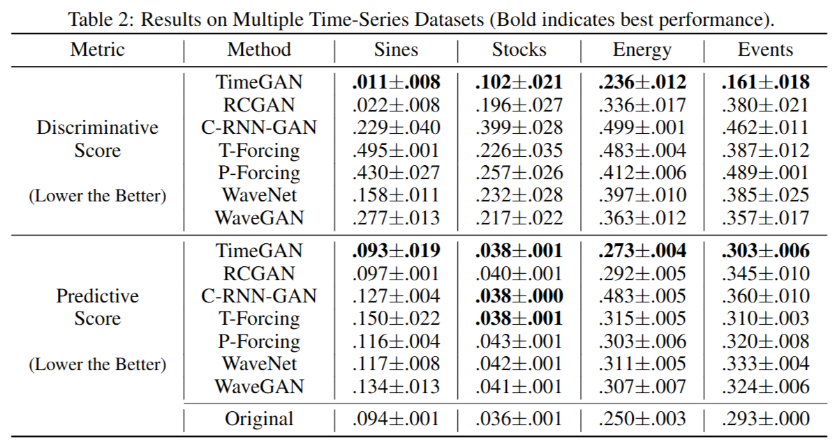
Benchmarks and Evaluation. We compare TimeGAN with RCGAN and C-RNN-GAN, the two most closely related methods. For purely autoregressive approaches, we compare against RNNs trained with teacher-forcing (T-Forcing) as well as professor-forcing (P-Forcing). For additional comparison, we consider the performance of WaveNet as well as its GAN counterpart WaveGAN. To assess the quality of generated data, we observe three desiderata: (1) diversity ---samples should be distributed to cover the real data; (2) fidelity ---samples should be indistinguishable from the real data; and (3) usefulness---samples should be just as useful as the real data when used for the same predictive purposes (i.e. train-on-synthetic, test-on-real).

(1) Visualization. We apply t-SNE and PCA analyses on both the original and synthetic datasets (flattening the temporal dimension). This visualizes how closely the distribution of generated samples resembles that of the original in 2-dimensional space, giving a qualitative assessment of (1).

(2) Discriminative Score. For a quantitative measure of similarity, we train a post-hoc time-series classification model (by optimizing a 2-layer LSTM) to distinguish between sequences from the original and generated datasets. First, each original sequence is labeled real , and each generated sequence is labeled not real. Then, an off-the-shelf (RNN) classifier is trained to distinguish between the two classes as a standard supervised task. We then report the classification error on the held-out test set, which gives a quantitative assessment of (2).

(3) Predictive Score. In order to be useful, the sampled data should inherit the predictive characteristics of the original. In particular, we expect TimeGAN to excel in capturing conditional distributions over time. Therefore, using the synthetic dataset, we train a post-hoc sequence-prediction model (by optimizing a 2-layer LSTM) to predict next-step temporal vectors over each input sequence. Then, we evaluate the trained model on the original dataset. Performance is measured in terms of the mean absolute error (MAE); for event-based data, the MAE is computed as |1 - estimated probability that the event occurred|. This gives a quantitative assessment of (3).

The Supplementary Materials contains additional information on benchmarks and hyperparameters, as well as further details of visualizations and hyperparameters for the post-hoc evaluation models. Implementation of TimeGAN can be found at https://bitbucket.org/mvdschaar/mlforhealthlabpub/src/master/alg/timegan/.

中文翻译:
基准与评估。 我们将 TimeGAN 与 RCGAN 和 C-RNN-GAN 这两个最相关的方法进行比较。对于纯自回归方法，我们与使用教师强制（T-Forcing）以及教授强制（P-Forcing）训练的 RNN 进行比较。作为补充比较，我们还考虑了 WaveNet 及其 GAN 对应版本 WaveGAN 的性能。为了评估生成数据的质量，我们遵循三个期望标准：(1) 多样性（diversity） ------样本分布应能覆盖真实数据；(2) 保真度（fidelity） ------样本应与真实数据难以区分；以及 (3) 实用性（usefulness）------当用于相同的预测目的时，样本应与真实数据同样有用（即，在合成数据上训练，在真实数据上测试）。

(1) 可视化。 我们对原始和合成数据集（将时间维度展平）同时应用 t-SNE 和 PCA 分析。这可以在二维空间中可视化生成样本的分布与原始分布的相似程度，从而对（1）多样性进行定性评估。

(2) 判别分数（Discriminative Score）。 为了定量衡量相似性，我们训练一个事后（post-hoc）时间序列分类模型（通过优化一个2层 LSTM）来区分来自原始数据集和生成数据集的序列。首先，每个原始序列被标记为 real ，每个生成序列被标记为 not real 。然后，训练一个现成的（RNN）分类器作为一个标准的监督任务来区分这两个类别。我们报告在留出测试集上的分类误差，这为（2）保真度提供了一个定量评估。（注：误差越低，说明生成数据和真实数据越难区分，模型性能越好。）

(3) 预测分数（Predictive Score）。 为了具有实用性，采样的数据应继承原始数据的预测特性。特别是，我们期望 TimeGAN 在捕捉随时间变化的条件分布方面表现出色。因此，我们使用合成数据集训练一个事后序列预测模型（通过优化一个2层 LSTM）来预测每个输入序列的下一步时间向量。然后，我们在原始数据集上评估这个训练好的模型。性能通过平均绝对误差（MAE）来衡量；对于基于事件的数据，MAE 计算为 |1 - 事件发生的估计概率|。这为（3）实用性提供了一个定量评估。（注：MAE 越低，说明生成数据保留的预测信息越多，模型性能越好。）

补充材料包含有关基准和超参数的更多信息，以及可视化和事后评估模型的更多细节。TimeGAN 的实现可以在 [链接] 找到。

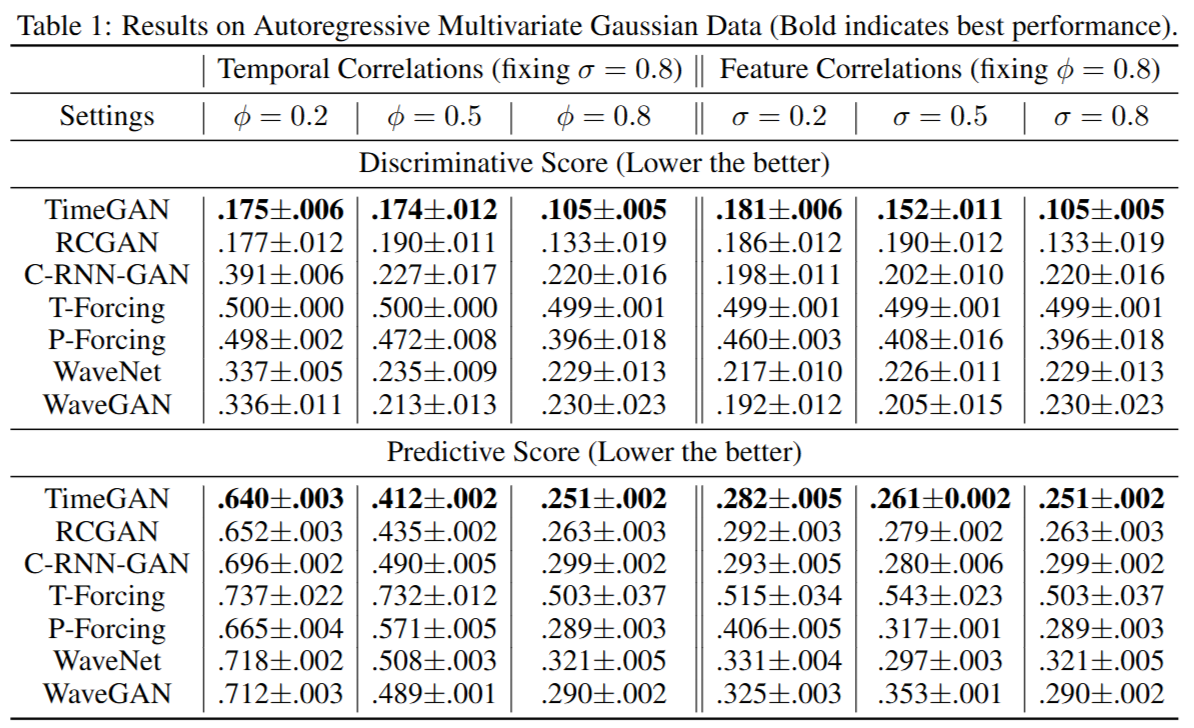
5.1 Illustrative Example: Autoregressive Gaussian Models

原文:

Our primary novelties are twofold: a supervised loss to better capture temporal dynamics, and an embedding network that provides a lower-dimensional adversarial learning space. To highlight these advantages, we experiment on sequences from autoregressive multivariate Gaussian models as follows: xt=ϕxt−1+n\mathbf{x}t = \phi \mathbf{x}{t-1} + \mathbf{n}xt=ϕxt−1+n, where n∼N(0,σ1+(1−σ)I)\mathbf{n} \sim \mathcal{N}(0, \sigma\mathbf{1} + (1-\sigma)\mathbf{I})n∼N(0,σ1+(1−σ)I). The coefficient ϕ∈\phi \inϕ∈ allows us to control the correlation across time steps, and σ∈[−1,1]\sigma \in [-1, 1]σ∈[−1,1] controls the correlation across features.

As shown in Table 1, TimeGAN consistently generates higher-quality synthetic data than benchmarks, in terms of both discriminative and predictive scores. This is true across the various settings for the underlying data-generating model. Importantly, observe that the advantage of TimeGAN is greater for higher settings of temporal correlation ϕ\phiϕ, lending credence to the motivation and benefit of the supervised loss mechanism. Likewise, observe that the advantage of TimeGAN is also greater for higher settings of feature correlation σ\sigmaσ, providing confirmation for the benefit of the embedding network.

中文翻译:

我们的主要创新点有两个：一个用于更好捕捉时间动态的监督损失，以及一个提供低维对抗学习空间的嵌入网络。为了凸显这些优势，我们在自回归多变量高斯模型生成的序列上进行实验，模型如下：xt=ϕxt−1+n\mathbf{x}t = \phi \mathbf{x}{t-1} + \mathbf{n}xt=ϕxt−1+n，其中 n∼N(0,σ1+(1−σ)I)\mathbf{n} \sim \mathcal{N}(0, \sigma\mathbf{1} + (1-\sigma)\mathbf{I})n∼N(0,σ1+(1−σ)I)。系数 ϕ∈\phi \inϕ∈ 允许我们控制跨时间步的相关性，而 σ∈[−1,1]\sigma \in [-1, 1]σ∈[−1,1] 控制特征间的相关性。

如表1所示，TimeGAN 在判别分数和预测分数方面，始终比基准模型生成更高质量的合成数据。这在数据生成模型的各种设置下都成立。重要的是，可以观察到，在时间相关性 ϕ\phiϕ 较高的设置中，TimeGAN 的优势更大，这证明了监督损失机制的动机和益处。同样地，可以观察到，在特征相关性 σ\sigmaσ 较高的设置中，TimeGAN 的优势也更大，这为嵌入网络的益处提供了证实。

5.2 Experiments on Different Types of Time Series Data

原文:

We test the performance of TimeGAN across time-series data with a variety of different characteristics, including periodicity, discreteness, level of noise, regularity of time steps, and correlation across time and features. The following datasets are selected on the basis of different combinations of these properties (detailed statistics of each dataset can be found in the Supplementary Materials).

(1) Sines. We simulate multivariate sinusoidal sequences of different frequencies η\etaη and phases θ\thetaθ, providing continuous-valued, periodic, multivariate data where each feature is independent of others. For each dimension i∈{1,...,5}i \in \{1, ..., 5\}i∈{1,...,5}, xi(t)=sin⁡(2πηit+θi)x_i(t) = \sin(2\pi\eta_i t + \theta_i)xi(t)=sin(2πηit+θi), where ηi∼U\eta_i \sim Uηi∼U and θi∼U[−π,π]\theta_i \sim U[-\pi, \pi]θi∼U[−π,π].

(2) Stocks. By contrast, sequences of stock prices are continuous-valued but aperiodic; furthermore, features are correlated with each other. We use the daily historical Google stocks data from 2004 to 2019, including as features the volume and high, low, opening, closing, and adjusted closing prices.

(3) Energy. Next, we consider a dataset characterized by noisy periodicity, higher dimensionality, and correlated features. The UCI Appliances energy prediction dataset consists of multivariate, continuous-valued measurements including numerous temporal features measured at close intervals.

(4) Events. Finally, we consider a dataset characterized by discrete values and irregular time stamps. We use a large private lung cancer pathways dataset consisting of sequences of events and their times, and model both the one-hot encoded sequence of event types as well as the event timings.

中文翻译:

我们在具有各种不同特征的时间序列数据上测试 TimeGAN 的性能，这些特征包括周期性、离散性、噪声水平、时间步的规律性以及跨时间和特征的相关性。根据这些属性的不同组合，我们选择了以下数据集（每个数据集的详细统计信息可在补充材料中找到）。

(1) 正弦波（Sines）。 我们模拟了不同频率 η\etaη 和相位 θ\thetaθ 的多变量正弦序列，提供连续值的、周期性的、多变量的数据，其中每个特征都相互独立。对于每个维度 i∈{1,...,5}i \in \{1, ..., 5\}i∈{1,...,5}，xi(t)=sin⁡(2πηit+θi)x_i(t) = \sin(2\pi\eta_i t + \theta_i)xi(t)=sin(2πηit+θi)，其中 ηi∼U\eta_i \sim Uηi∼U 和 θi∼U[−π,π]\theta_i \sim U[-\pi, \pi]θi∼U[−π,π]。

(2) 股票（Stocks）。 相比之下，股票价格序列是连续值的但非周期性的；此外，各特征之间相互关联。我们使用 2004 年至 2019 年的谷歌每日历史股票数据，特征包括成交量以及最高价、最低价、开盘价、收盘价和调整后收盘价。

(3) 能源（Energy）。 接下来，我们考虑一个具有噪声周期性、更高维度和相关特征的数据集。UCI 家用电器能耗预测数据集由多变量、连续值的测量数据组成，包括在很小的时间间隔内测量的众多时间特征。

(4) 事件（Events）。 最后，我们考虑一个具有离散值和不规则时间戳的数据集。我们使用一个大型的私人肺癌路径数据集，其中包含事件序列及其发生时间，我们同时对事件类型的 one-hot 编码序列和事件时间进行建模。

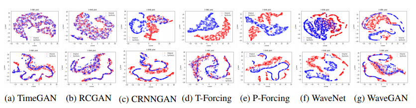
Figure 3: t-SNE visualization

原文（续）:

Visualizations with t-SNE and PCA. In Figure 3, we observe that synthetic datasets generated by TimeGAN show markedly better overlap with the original data than other benchmarks using t-SNE for visualization (PCA analysis can be found in the Supplementary Materials). In fact, we (in the first column) that the blue (generated) samples and red (original) samples are almost perfectly in sync.

Discriminative and Predictive Scores. As indicated in Table 2, TimeGAN consistently generates higher-quality synthetic data in comparison to benchmarks on the basis of both discriminative (post-hoc classification error) and predictive (mean absolute error) scores across all datasets. For instance for Stocks, TimeGAN-generated samples achieve 0.102 which is 48% lower than the next-best benchmark (RCGAN, at 0.196)---a statistically significant improvement. Remarkably, observe that the predictive scores of TimeGAN are almost on par with those of the original datasets themselves.

中文翻译（续）:
使用 t-SNE 和 PCA 的可视化。 在图3中，我们观察到使用 t-SNE 进行可视化时，由 TimeGAN 生成的合成数据集与原始数据的重叠程度明显优于其他基准模型（PCA 分析可在补充材料中找到）。事实上，我们（在第一列中）看到蓝色（生成的）样本和红色（原始的）样本几乎完美同步。

判别分数和预测分数。 如表2所示，在所有数据集上，基于判别（事后分类误差）和预测（平均绝对误差）分数，TimeGAN 始终比基准模型生成更高质量的合成数据。例如，对于股票数据，TimeGAN 生成的样本达到了 0.102 的判别分数，比次优基准（RCGAN，为 0.196）低 48%------这是一个统计上显著的改进。值得注意的是，TimeGAN 的预测分数几乎与原始数据集本身的预测分数相当。

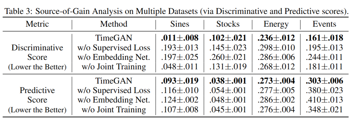
5.3 Sources of Gain

原文:

TimeGAN is characterized by (1) the supervised loss, (2) embedding networks, and (3) the joint training scheme. To analyze the importance of each contribution, we report the discriminative and predictive scores with the following modifications to TimeGAN: (1) without the supervised loss, (2) without the embedding networks, and (3) without jointly training the embedding and adversarial networks on the supervised loss. (The first corresponds to λ=η=0\lambda = \eta = 0λ=η=0, and the third to λ=0\lambda = 0λ=0).

We observe in Table 3 that all three elements make important contributions in improving the quality of the generated time-series data. The supervised loss plays a particularly important role when the data is characterized by high temporal correlations, such as in the Stocks dataset. In addition, we find that the embedding networks and joint training the with the adversarial networks (thereby aligning the targets of the two) clearly and consistently improves generative performance across the board.

中文翻译:

TimeGAN 的特点是 (1) 监督损失，(2) 嵌入网络，和 (3) 联合训练方案。为了分析每个贡献的重要性，我们报告了对 TimeGAN 进行以下修改后的判别和预测分数：(1) 去除监督损失，(2) 去除嵌入网络，和 (3) 在监督损失上不联合训练嵌入和对抗网络。（第一个对应于 λ=η=0\lambda = \eta = 0λ=η=0，第三个对应于 λ=0\lambda = 0λ=0）。

我们在表3中观察到，所有三个元素都在提高生成的时间序列数据质量方面做出了重要贡献。当数据具有高时间相关性时，例如在股票数据集中，监督损失扮演了尤其重要的角色。此外，我们发现嵌入网络以及与对抗网络的联合训练（从而统一了两者的目标）在所有情况下都清晰且一致地提高了生成性能。

6 Conclusion (结论)

原文:

In this paper we introduce TimeGAN, a novel framework for time-series generation that combines the versatility of the unsupervised GAN approach with the control over conditional temporal dynamics afforded by supervised autoregressive models. Leveraging the contributions of the supervised loss and jointly trained embedding network, TimeGAN demonstrates consistent and significant improvements over state-of-the-art benchmarks in generating realistic time-series data. In the future, further work may investigate incorporating the differential privacy framework into the TimeGAN approach in order to generate high-quality time-series data with differential privacy guarantees.

中文翻译:

在本文中，我们介绍了 TimeGAN，一个用于时间序列生成的新颖框架，它结合了无监督 GAN 方法的多功能性与监督自回归模型所提供的对条件时间动态的控制力。通过利用监督损失和联合训练的嵌入网络的贡献，TimeGAN 在生成逼真的时间序列数据方面，展示了相比于最先进基准的一致且显著的改进。未来，进一步的工作可以研究将差分隐私框架整合到 TimeGAN 方法中，以生成具有差分隐私保证的高质量时间序列数据。

💡 解读:

结论部分简洁地重申了 TimeGAN 的核心贡献：

方法论创新: 成功地将无监督 GAN 的生成能力与有监督自回归模型的时序控制能力结合。
关键技术 : 强调了监督损失 (LS\mathcal{L}_SLS) 和联合训练的嵌入网络是实现这一目标的核心。
成果: 实验证明模型效果优于现有 SOTA (State-of-the-Art) 模型。
未来展望 (Future Work) : 提出了一个非常有价值的研究方向------差分隐私 (Differential Privacy)。这意味着他们希望未来的 TimeGAN 不仅能生成逼真的数据，还能在生成过程中保护原始数据中的个人隐私，这在医疗、金融等敏感领域至关重要。

TimeGAN论文精读