
引言
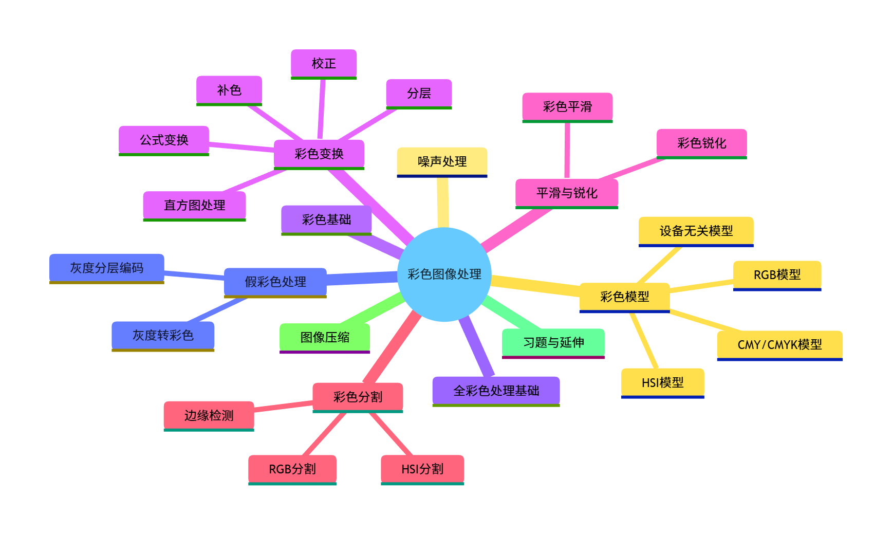
在数字图像处理领域,彩色图像处理是极具实用性的分支。相较于灰度图像,彩色图像能携带更丰富的视觉信息,广泛应用于遥感监测、医学影像、工业检测、自动驾驶等场景。本章将从彩色基础理论出发,逐步讲解彩色模型、各类彩色图像处理技术,并结合可直接运行的 Python 代码实现效果可视化,让大家从理论到实践吃透彩色图像处理。
学习目标
- 理解彩色的物理和视觉基础,掌握主流彩色模型的原理及相互转换方法
- 掌握假彩色图像处理、全彩色图像处理的核心思路
- 学会彩色变换、平滑、锐化、分割等常用处理技术的实现
- 理解彩色图像噪声处理和压缩的基本原理
- 能够使用 Python 实现各类彩色图像处理算法,并分析处理效果
6.1 彩色基础
彩色视觉的本质是人类视觉系统对可见光波段(380~780nm)电磁波的感知。从物理角度,彩色由亮度(Luminance) 、色调(Hue) 、饱和度(Saturation) 三个特征描述:
- 亮度:光的强度,对应灰度图像的灰度值
- 色调:区分不同颜色的特征(如红、绿、蓝)
- 饱和度:颜色的纯净度,饱和度越高颜色越鲜艳
6.2 彩色模型
彩色模型(颜色空间)是用数值表示颜色的规范,不同模型适用于不同场景。
6.2.1 RGB 彩色模型
RGB 模型是加色模型,基于红、绿、蓝三原色叠加生成颜色,是计算机显示、数字图像的核心模型(如显示器、相机传感器)。
- 取值范围:每个通道 0~255(8 位),(0,0,0) 为黑,(255,255,255) 为白
- 原理:红绿蓝
代码实现:RGB 模型可视化及通道分离
import cv2
import numpy as np
import matplotlib.pyplot as plt

# 设置matplotlib支持中文显示
plt.rcParams['font.sans-serif'] = ['SimHei']  # 黑体
plt.rcParams['axes.unicode_minus'] = False    # 解决负号显示问题

# 1. 创建纯RGB颜色示例
def create_rgb_color():
    # 创建红色、绿色、蓝色、黄色(红+绿)、洋红(红+蓝)、青色(绿+蓝)、白色、黑色
    colors = {
        '红色': (255, 0, 0),
        '绿色': (0, 255, 0),
        '蓝色': (0, 0, 255),
        '黄色': (255, 255, 0),
        '洋红': (255, 0, 255),
        '青色': (0, 255, 255),
        '白色': (255, 255, 255),
        '黑色': (0, 0, 0)
    }
    # 创建画布
    canvas = np.zeros((200, len(colors)*100, 3), dtype=np.uint8)
    for i, (name, rgb) in enumerate(colors.items()):
        canvas[:, i*100:(i+1)*100, :] = rgb
    return canvas, colors

# 2. 读取图像并分离RGB通道
def rgb_channel_split(img_path):
    # 读取图像(OpenCV默认BGR,转换为RGB)
    img_bgr = cv2.imread(img_path)
    img_rgb = cv2.cvtColor(img_bgr, cv2.COLOR_BGR2RGB)

    # 分离通道
    r_channel = img_rgb[:, :, 0]
    g_channel = img_rgb[:, :, 1]
    b_channel = img_rgb[:, :, 2]

    # 生成单通道可视化图(其他通道置0)
    r_img = np.zeros_like(img_rgb)
    r_img[:, :, 0] = r_channel
    g_img = np.zeros_like(img_rgb)
    g_img[:, :, 1] = g_channel
    b_img = np.zeros_like(img_rgb)
    b_img[:, :, 2] = b_channel

    return img_rgb, r_img, g_img, b_img, r_channel, g_channel, b_channel

# 主执行逻辑
if __name__ == "__main__":
    # 生成RGB基础颜色示例
    rgb_color_canvas, _ = create_rgb_color()

    # 读取测试图像(替换为你的图像路径)
    img_path = "test.jpg"  # 建议使用彩色风景/人物图
    try:
        img_rgb, r_img, g_img, b_img, r_chan, g_chan, b_chan = rgb_channel_split(img_path)
    except:
        print("图像读取失败,请检查路径!")
        # 生成测试图像
        img_rgb = np.random.randint(0, 255, (300, 400, 3), dtype=np.uint8)
        r_img, g_img, b_img = np.zeros_like(img_rgb), np.zeros_like(img_rgb), np.zeros_like(img_rgb)
        r_img[:, :, 0] = img_rgb[:, :, 0]
        g_img[:, :, 1] = img_rgb[:, :, 1]
        b_img[:, :, 2] = img_rgb[:, :, 2]

    # 可视化1:RGB基础颜色
    plt.figure(figsize=(12, 3))
    plt.imshow(rgb_color_canvas)
    plt.title('RGB基础颜色示例')
    plt.axis('off')
    plt.show()

    # 可视化2:RGB通道分离
    plt.figure(figsize=(15, 10))
    plt.subplot(2, 2, 1)
    plt.imshow(img_rgb)
    plt.title('原始RGB图像')
    plt.axis('off')

    plt.subplot(2, 2, 2)
    plt.imshow(r_img)
    plt.title('R通道')
    plt.axis('off')

    plt.subplot(2, 2, 3)
    plt.imshow(g_img)
    plt.title('G通道')
    plt.axis('off')

    plt.subplot(2, 2, 4)
    plt.imshow(b_img)
    plt.title('B通道')
    plt.axis('off')
    plt.show()

    # 可视化3:通道灰度图
    plt.figure(figsize=(15, 5))
    plt.subplot(1, 3, 1)
    plt.imshow(r_chan, cmap='gray')
    plt.title('R通道灰度图')
    plt.axis('off')

    plt.subplot(1, 3, 2)
    plt.imshow(g_chan, cmap='gray')
    plt.title('G通道灰度图')
    plt.axis('off')

    plt.subplot(1, 3, 3)
    plt.imshow(b_chan, cmap='gray')
    plt.title('B通道灰度图')
    plt.axis('off')
    plt.show()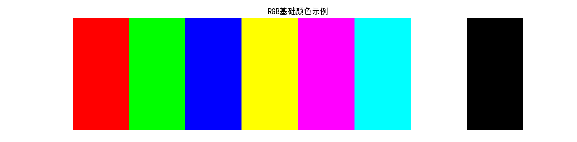
效果说明
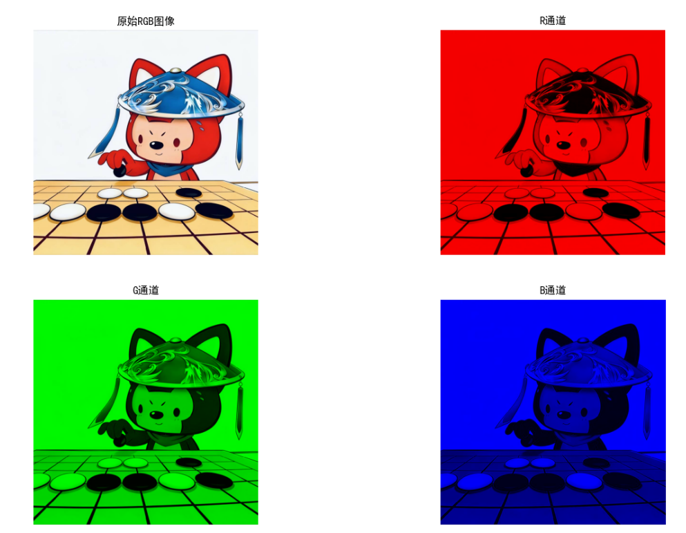
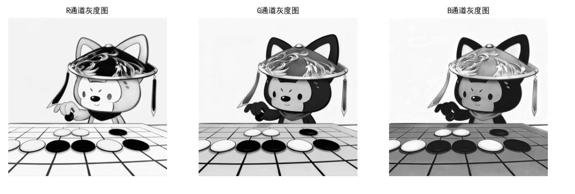
运行代码后会显示 3 组图:
- RGB 基础颜色面板:直观看到三原色及混合色效果
- 彩色图像的 RGB 单通道彩色可视化:每个通道单独显示为对应颜色
- 通道灰度图:每个通道的亮度分布(灰度值越高,该通道颜色越浓)
6.2.2 CMY 和 CMYK 彩色模型
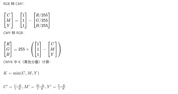
CMY 模型是减色模型,基于青(Cyan)、品红(Magenta)、黄(Yellow)三原色,适用于印刷、打印场景(墨水吸收光)。CMYK 在 CMY 基础上增加了黑色(Key),解决 CMY 混合无法生成纯黑的问题。
数学转换
代码实现:RGB 与 CMY/CMYK 转换
import cv2
import numpy as np
import matplotlib.pyplot as plt

plt.rcParams['font.sans-serif'] = ['SimHei']
plt.rcParams['axes.unicode_minus'] = False

# RGB转CMY
def rgb_to_cmy(img_rgb):
    # 归一化到0-1
    rgb_norm = img_rgb / 255.0
    # CMY计算
    c = 1 - rgb_norm[:, :, 0]
    m = 1 - rgb_norm[:, :, 1]
    y = 1 - rgb_norm[:, :, 2]
    # 合并为CMY图像(转换为0-255)
    cmy_img = np.stack([c, m, y], axis=-1) * 255
    cmy_img = cmy_img.astype(np.uint8)
    return cmy_img, c, m, y

# CMY转CMYK
def cmy_to_cmyk(c, m, y):
    # 计算K分量
    k = np.min(np.stack([c, m, y], axis=-1), axis=-1)
    # 避免除以0
    k = np.where(k == 1, 0.9999, k)
    # 计算CMY'
    c_prime = (c - k) / (1 - k)
    m_prime = (m - k) / (1 - k)
    y_prime = (y - k) / (1 - k)
    # 转换为0-255
    cmyk_img = np.stack([c_prime, m_prime, y_prime, k], axis=-1) * 255
    cmyk_img = cmyk_img.astype(np.uint8)
    return cmyk_img, k

# CMYK转RGB
def cmyk_to_rgb(cmyk_img):
    cmyk_norm = cmyk_img / 255.0
    c, m, y, k = cmyk_norm[:, :, 0], cmyk_norm[:, :, 1], cmyk_norm[:, :, 2], cmyk_norm[:, :, 3]
    # 先转CMY
    c = c * (1 - k) + k
    m = m * (1 - k) + k
    y = y * (1 - k) + k
    # 再转RGB
    rgb_norm = 1 - np.stack([c, m, y], axis=-1)
    rgb_img = (rgb_norm * 255).astype(np.uint8)
    return rgb_img

# 主执行
if __name__ == "__main__":
    # 读取图像
    img_path = "test.jpg"
    img_bgr = cv2.imread(img_path)
    img_rgb = cv2.cvtColor(img_bgr, cv2.COLOR_BGR2RGB)

    # RGB转CMY
    cmy_img, c, m, y = rgb_to_cmy(img_rgb)
    # CMY转CMYK
    cmyk_img, k = cmy_to_cmyk(c, m, y)
    # CMYK转回RGB
    rgb_recon = cmyk_to_rgb(cmyk_img)

    # 可视化
    plt.figure(figsize=(18, 12))

    # 原始RGB
    plt.subplot(2, 3, 1)
    plt.imshow(img_rgb)
    plt.title('原始RGB图像')
    plt.axis('off')

    # CMY图像
    plt.subplot(2, 3, 2)
    plt.imshow(cmy_img)
    plt.title('CMY图像')
    plt.axis('off')

    # CMYK图像(显示前3通道)
    plt.subplot(2, 3, 3)
    plt.imshow(cmyk_img[:, :, :3])
    plt.title('CMYK图像(CMY分量)')
    plt.axis('off')

    # K分量灰度图
    plt.subplot(2, 3, 4)
    plt.imshow(k, cmap='gray')
    plt.title('CMYK-K分量(黑色)')
    plt.axis('off')

    # 还原的RGB图像
    plt.subplot(2, 3, 5)
    plt.imshow(rgb_recon)
    plt.title('CMYK转回RGB图像')
    plt.axis('off')

    # 误差图(原始-还原)
    error = np.abs(img_rgb - rgb_recon)
    plt.subplot(2, 3, 6)
    plt.imshow(error, cmap='gray')
    plt.title('转换误差(灰度)')
    plt.axis('off')

    plt.tight_layout()
    plt.show()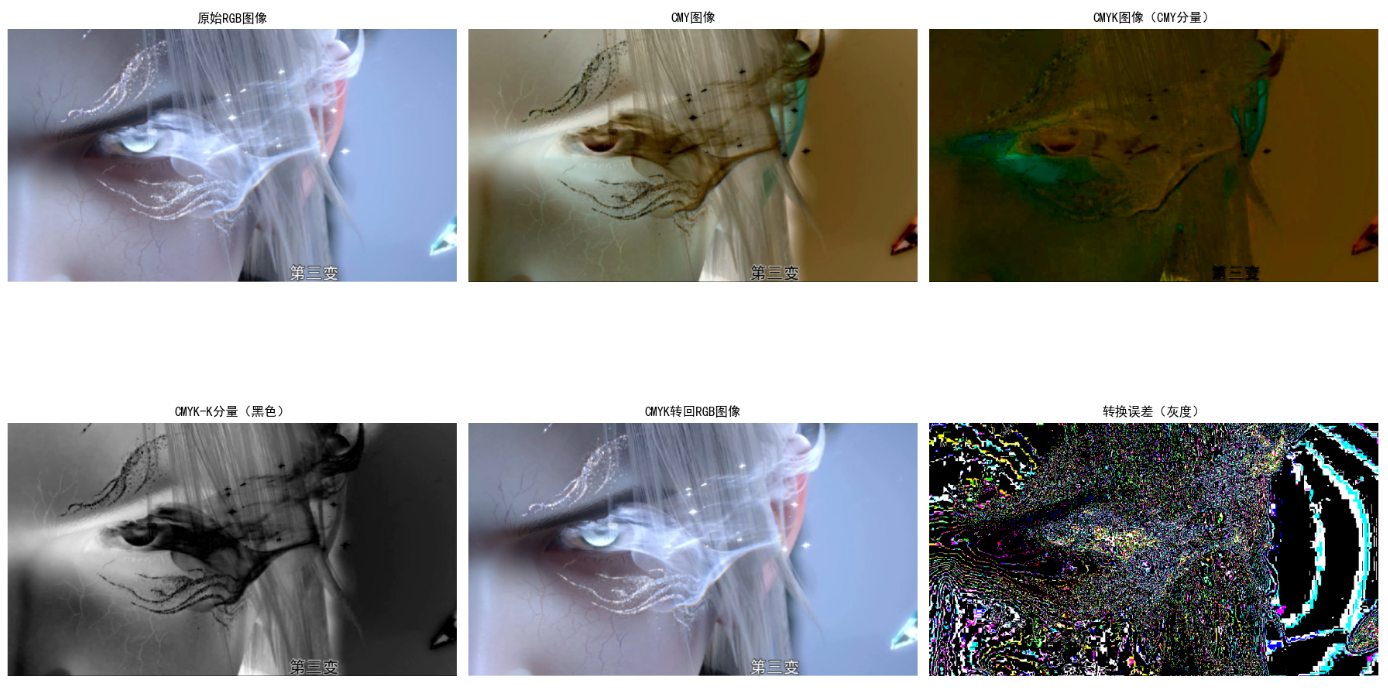
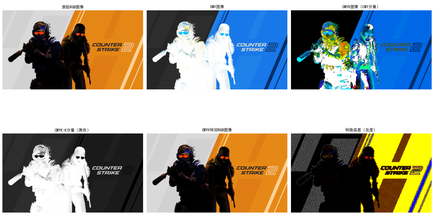
效果说明
- CMY 图像:颜色与 RGB 互补(如 RGB 红色对应 CMY 青色)
- K 分量图:越亮的区域黑色墨水越多
- 还原 RGB 与原始图像几乎无差异,验证转换公式正确性
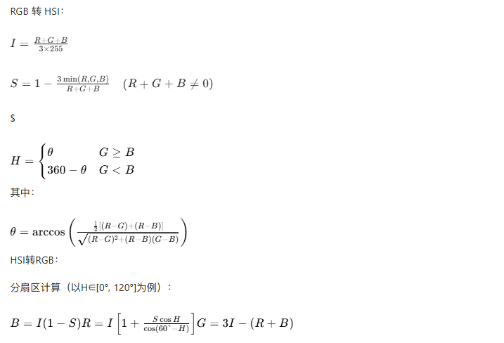
6.2.3 HSI 彩色模型
HSI 模型直接对应人类对颜色的感知(色调 H、饱和度 S、亮度 I),是彩色图像处理的核心模型(如颜色分割、校正)。
- 色调 H:0~360°(0° 红、120° 绿、240° 蓝)
- 饱和度 S:0~1(0 为灰度,1 为纯颜色)
- 亮度 I:0~1(0 黑,1 白)
数学转换
代码实现:RGB与HSI转换及可视化
import cv2
import numpy as np
import matplotlib.pyplot as plt
import math

plt.rcParams['font.sans-serif'] = ['SimHei']
plt.rcParams['axes.unicode_minus'] = False

# RGB转HSI
def rgb_to_hsi(img_rgb):
    # 归一化到0-1
    r = img_rgb[:, :, 0] / 255.0
    g = img_rgb[:, :, 1] / 255.0
    b = img_rgb[:, :, 2] / 255.0

    # 计算亮度I
    i = (r + g + b) / 3.0

    # 计算饱和度S
    min_rgb = np.min(np.stack([r, g, b], axis=-1), axis=-1)
    s = 1 - 3 * min_rgb / (r + g + b + 1e-6)  # 避免除0
    s = np.where(r + g + b == 0, 0, s)  # 黑色时S=0

    # 计算色调H
    num = 0.5 * ((r - g) + (r - b))
    den = np.sqrt((r - g)**2 + (r - b)*(g - b)) + 1e-6
    theta = np.arccos(num / den)
    h = np.where(b > g, 2 * np.pi - theta, theta)
    h = h / (2 * np.pi)  # 归一化到0-1

    # 合并HSI
    hsi_img = np.stack([h, s, i], axis=-1)
    return hsi_img, h, s, i

# HSI转RGB
def hsi_to_rgb(hsi_img):
    h = hsi_img[:, :, 0] * 2 * np.pi  # 转回弧度
    s = hsi_img[:, :, 1]
    i = hsi_img[:, :, 2]

    r, g, b = np.zeros_like(h), np.zeros_like(h), np.zeros_like(h)

    # 扇区1: 0 <= H < 120°
    mask1 = (h >= 0) & (h < 2 * np.pi / 3)
    h1 = h[mask1]
    s1 = s[mask1]
    i1 = i[mask1]
    b1 = i1 * (1 - s1)
    r1 = i1 * (1 + s1 * np.cos(h1) / np.cos(np.pi/3 - h1))
    g1 = 3 * i1 - (r1 + b1)
    r[mask1] = r1
    g[mask1] = g1
    b[mask1] = b1

    # 扇区2: 120° <= H < 240°
    mask2 = (h >= 2 * np.pi / 3) & (h < 4 * np.pi / 3)
    h2 = h[mask2] - 2 * np.pi / 3
    s2 = s[mask2]
    i2 = i[mask2]
    r2 = i2 * (1 - s2)
    g2 = i2 * (1 + s2 * np.cos(h2) / np.cos(np.pi/3 - h2))
    b2 = 3 * i2 - (r2 + g2)
    r[mask2] = r2
    g[mask2] = g2
    b[mask2] = b2

    # 扇区3: 240° <= H < 360°
    mask3 = (h >= 4 * np.pi / 3) & (h < 2 * np.pi)
    h3 = h[mask3] - 4 * np.pi / 3
    s3 = s[mask3]
    i3 = i[mask3]
    g3 = i3 * (1 - s3)
    b3 = i3 * (1 + s3 * np.cos(h3) / np.cos(np.pi/3 - h3))
    r3 = 3 * i3 - (g3 + b3)
    r[mask3] = r3
    g[mask3] = g3
    b[mask3] = b3

    # 归一化到0-255
    rgb_img = np.stack([r, g, b], axis=-1)
    rgb_img = np.clip(rgb_img, 0, 1) * 255
    rgb_img = rgb_img.astype(np.uint8)
    return rgb_img

# 主执行
if __name__ == "__main__":
    # 读取图像
    img_path = "test.jpg"
    img_bgr = cv2.imread(img_path)
    img_rgb = cv2.cvtColor(img_bgr, cv2.COLOR_BGR2RGB)

    # RGB转HSI
    hsi_img, h, s, i = rgb_to_hsi(img_rgb)
    # HSI转RGB
    rgb_recon = hsi_to_rgb(hsi_img)

    # 可视化HSI分量
    plt.figure(figsize=(18, 10))

    # 原始RGB
    plt.subplot(2, 4, 1)
    plt.imshow(img_rgb)
    plt.title('原始RGB图像')
    plt.axis('off')

    # H分量(色调)
    plt.subplot(2, 4, 2)
    plt.imshow(h, cmap='hsv')
    plt.title('H分量(色调)')
    plt.axis('off')

    # S分量(饱和度)
    plt.subplot(2, 4, 3)
    plt.imshow(s, cmap='gray')
    plt.title('S分量(饱和度)')
    plt.axis('off')

    # I分量(亮度)
    plt.subplot(2, 4, 4)
    plt.imshow(i, cmap='gray')
    plt.title('I分量(亮度)')
    plt.axis('off')

    # HSI图像(伪彩色)
    plt.subplot(2, 4, 5)
    plt.imshow(hsi_img)
    plt.title('HSI图像(伪彩色)')
    plt.axis('off')

    # 还原的RGB图像
    plt.subplot(2, 4, 6)
    plt.imshow(rgb_recon)
    plt.title('HSI转回RGB图像')
    plt.axis('off')

    # 误差图
    error = np.abs(img_rgb - rgb_recon)
    plt.subplot(2, 4, 7)
    plt.imshow(error, cmap='gray')
    plt.title('转换误差(灰度)')
    plt.axis('off')

    # 误差直方图
    plt.subplot(2, 4, 8)
    plt.hist(error.flatten(), bins=50, color='gray')
    plt.title('转换误差分布')
    plt.xlabel('误差值')
    plt.ylabel('像素数')

    plt.tight_layout()
    plt.show()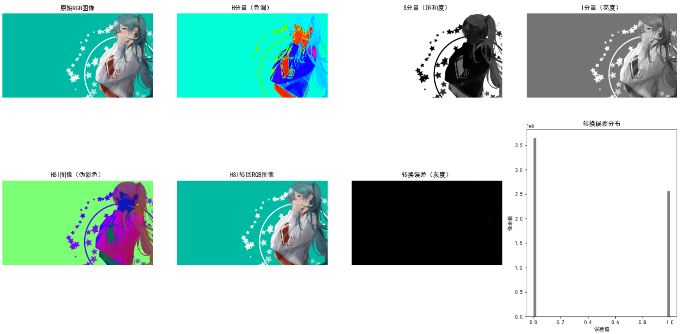
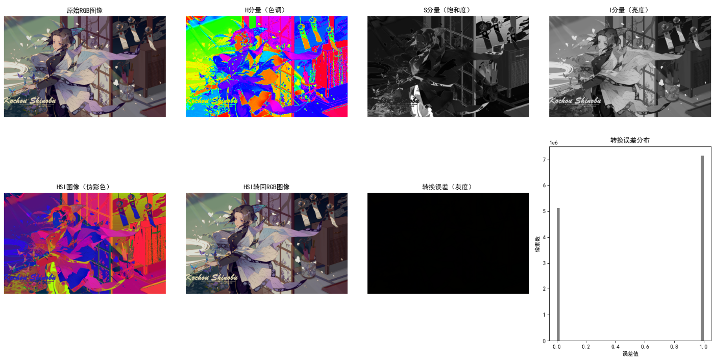
效果说明
- H分量图:不同颜色区域呈现不同色调值,直观区分颜色类别
- S分量图:越亮的区域颜色越鲜艳,暗区为灰度/低饱和度
- I分量图:等价于RGB的亮度灰度图
- 还原RGB与原始图像几乎无差异,验证转换准确性
6.2.4 设备无关彩色模型
设备无关模型(如CIE XYZ、CIE Lab、CIE Luv)解决不同设备颜色显示不一致的问题,是颜色标准化的基础。
CIE XYZ模型(MathType格式)
RGB转CIE XYZ:

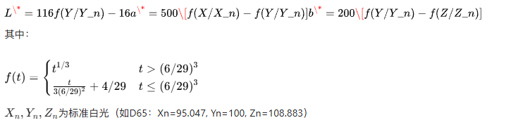
CIE Lab模型
代码实现:RGB转CIE Lab
python
import cv2
import numpy as np
import matplotlib.pyplot as plt
import matplotlib.cm as cm

# ========== 1. 基础配置 ==========
# 设置中文显示
plt.rcParams['font.sans-serif'] = ['SimHei']
plt.rcParams['axes.unicode_minus'] = False

# ========== 2. 打印可用Colormap(验证) ==========
print("Matplotlib支持的Colormap列表:")
cmap_list = sorted(cm.datad)
for cmap_name in cmap_list:
    print(cmap_name)
print("-" * 50)


# ========== 3. 颜色空间转换函数 ==========
# RGB转XYZ
def rgb_to_xyz(img_rgb):
    # 归一化到0-1
    rgb_norm = img_rgb / 255.0
    # 伽马校正(sRGB标准)
    rgb_norm = np.where(rgb_norm > 0.04045, ((rgb_norm + 0.055) / 1.055) ** 2.4, rgb_norm / 12.92)
    # XYZ转换矩阵(D65光源)
    transform_mat = np.array([
        [0.412453, 0.357580, 0.180423],
        [0.212671, 0.715160, 0.072169],
        [0.019334, 0.119193, 0.950227]
    ])
    # 矩阵乘法(展平后计算,再还原形状)
    xyz = np.dot(rgb_norm.reshape(-1, 3), transform_mat.T).reshape(img_rgb.shape)
    return xyz


# XYZ转Lab
def xyz_to_lab(xyz_img):
    # 标准白光D65的参考值
    Xn = 95.047
    Yn = 100.0
    Zn = 108.883

    # 归一化到参考白
    x = xyz_img[:, :, 0] / Xn
    y = xyz_img[:, :, 1] / Yn
    z = xyz_img[:, :, 2] / Zn

    # Lab转换核心函数
    def f(t):
        threshold = (6 / 29) ** 3
        return np.where(t > threshold, t ** (1 / 3), (t * 3 * (6 / 29) ** 2) + 4 / 29)

    fx = f(x)
    fy = f(y)
    fz = f(z)

    # 计算Lab分量
    L = 116 * fy - 16
    a = 500 * (fx - fy)
    b = 200 * (fy - fz)

    # 归一化到0-255(便于图像显示)
    L_norm = np.clip((L / 100) * 255, 0, 255).astype(np.uint8)
    a_norm = np.clip(((a + 128) / 256) * 255, 0, 255).astype(np.uint8)
    b_norm = np.clip(((b + 128) / 256) * 255, 0, 255).astype(np.uint8)

    lab_img = np.stack([L_norm, a_norm, b_norm], axis=-1)
    return lab_img, L, a, b


# ========== 4. 主执行逻辑 ==========
if __name__ == "__main__":
    # 读取图像(兼容路径错误)
    img_path = "../picture/1.jpg"  # 替换为你的图像路径
    img_bgr = cv2.imread(img_path)

    # 若图像读取失败,生成测试图像
    if img_bgr is None:
        print(f"未找到图像文件:{img_path},自动生成测试图像")
        img_rgb = np.random.randint(0, 255, (400, 600, 3), dtype=np.uint8)
    else:
        img_rgb = cv2.cvtColor(img_bgr, cv2.COLOR_BGR2RGB)  # 转换为RGB格式

    # 执行颜色空间转换
    xyz_img = rgb_to_xyz(img_rgb)
    lab_img, L_channel, a_channel, b_channel = xyz_to_lab(xyz_img)

    # ========== 5. 可视化结果 ==========
    plt.figure(figsize=(16, 12))

    # 原始RGB图像
    plt.subplot(2, 2, 1)
    plt.imshow(img_rgb)
    plt.title("原始RGB图像", fontsize=12)
    plt.axis("off")

    # Lab-L分量(亮度)
    plt.subplot(2, 2, 2)
    plt.imshow(L_channel, cmap="gray")
    plt.title("Lab-L分量(亮度)", fontsize=12)
    plt.axis("off")

    # Lab-a分量(红-绿轴)
    plt.subplot(2, 2, 3)
    plt.imshow(a_channel, cmap="RdBu")  # 红-蓝配色,对应红-绿
    plt.title("Lab-a分量(红→绿)", fontsize=12)
    plt.axis("off")

    # Lab-b分量(黄-蓝轴)
    plt.subplot(2, 2, 4)
    plt.imshow(b_channel, cmap="YlGnBu")  # 黄-绿-蓝配色,对应黄-蓝
    plt.title("Lab-b分量(黄→蓝)", fontsize=12)
    plt.axis("off")

    # 调整布局并显示
    plt.tight_layout()
    plt.show()

    print("程序执行完成!")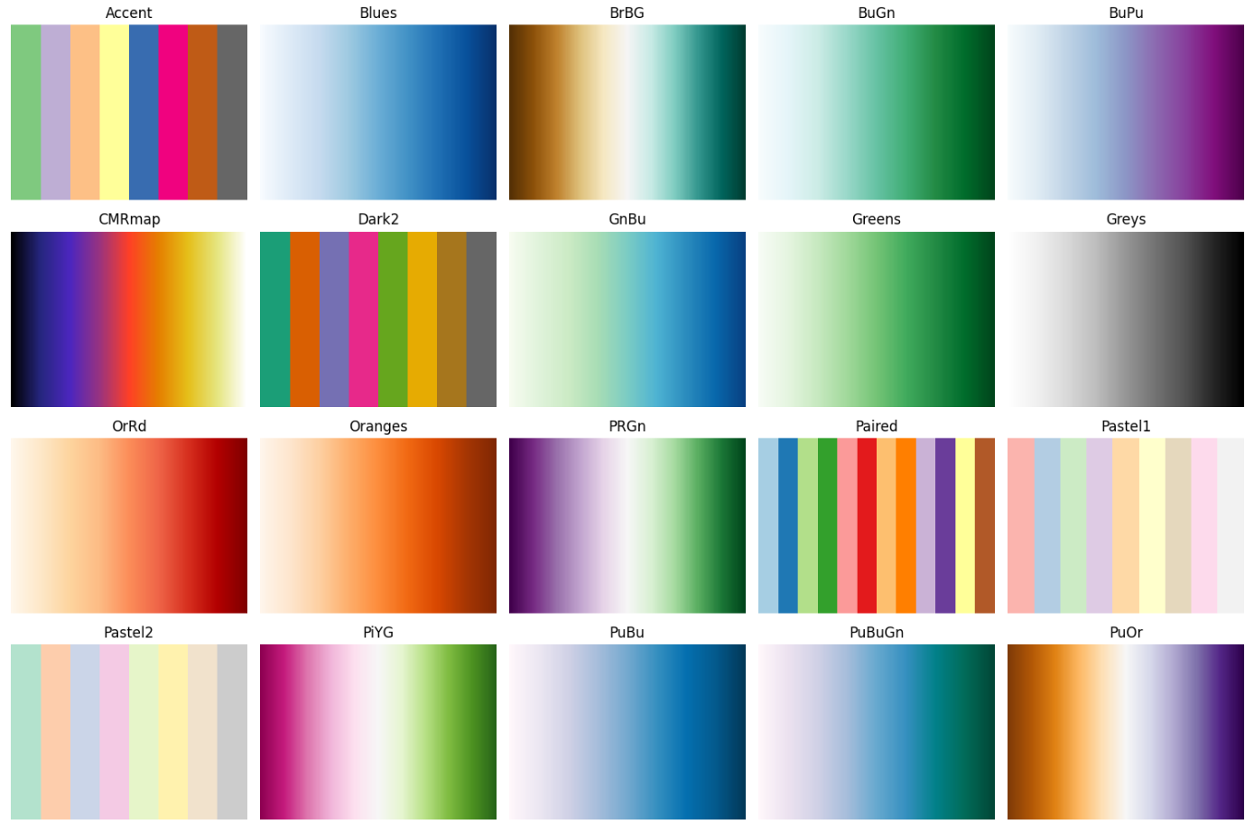
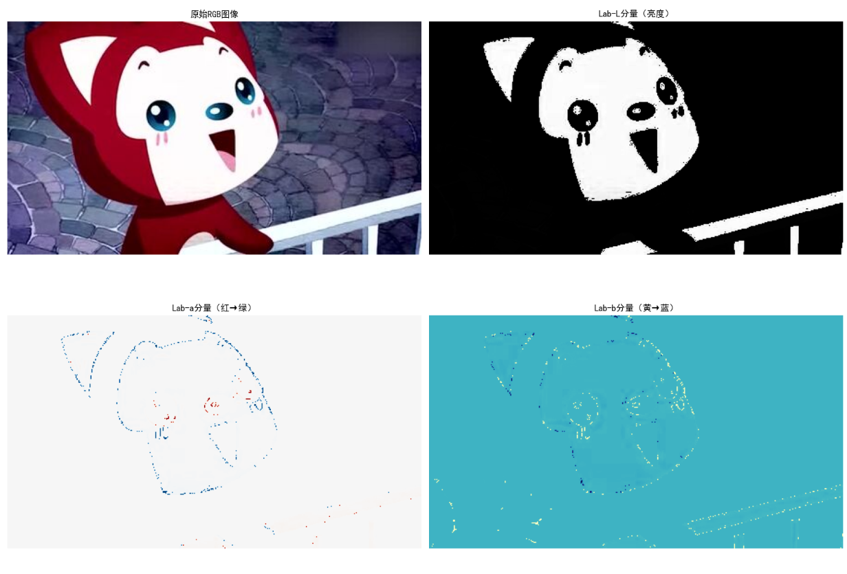
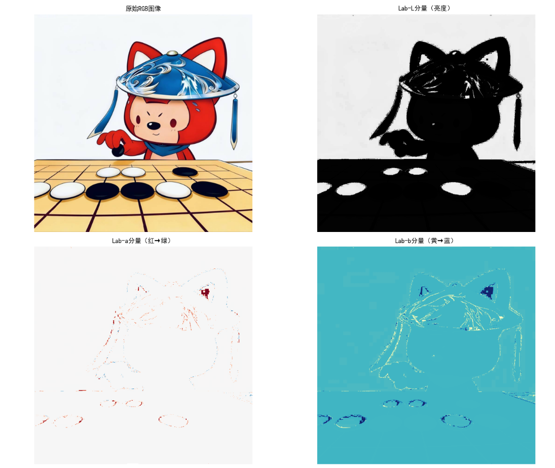
效果说明
- L分量:亮度信息,与人类视觉感知一致
- a分量:红-绿轴,正值偏红,负值偏绿
- b分量:黄-蓝轴,正值偏黄,负值偏蓝
6.3 假彩色图像处理
假彩色处理是将灰度图像/单波段图像转换为彩色图像,增强视觉辨识度,适用于医学影像、遥感图像等场景。
6.3.1 灰度分层和彩色编码
灰度分层(密度分割):将灰度值划分为若干区间,每个区间赋予不同颜色。
代码实现:灰度分层彩色编码
import cv2
import numpy as np
import matplotlib.pyplot as plt

plt.rcParams['font.sans-serif'] = ['SimHei']
plt.rcParams['axes.unicode_minus'] = False

# 灰度分层彩色编码
def gray_layer_color(gray_img, layers=8):
    # 计算分层阈值
    thresholds = np.linspace(0, 255, layers+1)
    # 创建彩色图像
    color_img = np.zeros((gray_img.shape[0], gray_img.shape[1], 3), dtype=np.uint8)

    # 定义颜色映射(可自定义)
    colors = [
        (0, 0, 255),    # 蓝
        (0, 128, 255),  # 浅蓝
        (0, 255, 255),  # 青
        (0, 255, 0),    # 绿
        (255, 255, 0),  # 黄
        (255, 128, 0),  # 橙
        (255, 0, 0),    # 红
        (128, 0, 255)   # 紫
    ]

    # 分层赋值
    for i in range(layers):
        mask = (gray_img >= thresholds[i]) & (gray_img < thresholds[i+1])
        color_img[mask] = colors[i]

    # 处理最大值(255)
    color_img[gray_img == 255] = colors[-1]

    return color_img, thresholds

# 主执行
if __name__ == "__main__":
    # 读取灰度图像(或彩色转灰度)
    img_path = "test.jpg"
    img_bgr = cv2.imread(img_path)
    gray_img = cv2.cvtColor(img_bgr, cv2.COLOR_BGR2GRAY)

    # 灰度分层(8层)
    color_layer_8, _ = gray_layer_color(gray_img, layers=8)
    # 灰度分层(4层)
    color_layer_4, _ = gray_layer_color(gray_img, layers=4)

    # 可视化
    plt.figure(figsize=(15, 5))

    plt.subplot(1, 3, 1)
    plt.imshow(gray_img, cmap='gray')
    plt.title('原始灰度图像')
    plt.axis('off')

    plt.subplot(1, 3, 2)
    plt.imshow(color_layer_4)
    plt.title('4层灰度分层编码')
    plt.axis('off')

    plt.subplot(1, 3, 3)
    plt.imshow(color_layer_8)
    plt.title('8层灰度分层编码')
    plt.axis('off')

    plt.tight_layout()
    plt.show()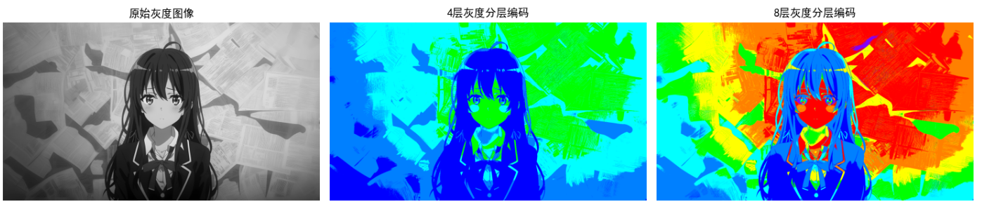
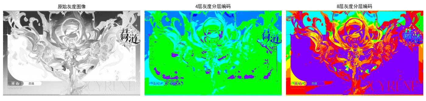
效果说明
- 分层数越多,颜色细节越丰富
- 低灰度值(暗区)显示冷色调,高灰度值(亮区)显示暖色调,直观区分不同亮度区域
6.3.2 灰度到彩色的变换
通过映射函数将灰度值转换为RGB值,常用的有伪彩色映射(如jet、viridis)。
代码实现:灰度到彩色的自定义映射
import cv2
import numpy as np
import matplotlib.pyplot as plt
from matplotlib import cm

plt.rcParams['font.sans-serif'] = ['SimHei']
plt.rcParams['axes.unicode_minus'] = False

# 自定义灰度到彩色映射
def gray_to_color_custom(gray_img):
    # 创建映射表
    color_map = np.zeros((256, 3), dtype=np.uint8)

    # 红通道:0-127→0-255,128-255→255-0
    color_map[:, 0] = np.concatenate([np.linspace(0, 255, 128), np.linspace(255, 0, 128)])
    # 绿通道:0-63→0-255,64-191→255,192-255→255-0
    green = np.concatenate([np.linspace(0, 255, 64), np.full(128, 255), np.linspace(255, 0, 64)])
    color_map[:, 1] = green
    # 蓝通道:0-127→255-0,128-255→0-255
    color_map[:, 2] = np.concatenate([np.linspace(255, 0, 128), np.linspace(0, 255, 128)])

    # 应用映射
    color_img = color_map[gray_img]
    return color_img

# 使用matplotlib内置映射
def gray_to_color_matplotlib(gray_img, cmap_name='jet'):
    # 归一化灰度图
    gray_norm = gray_img / 255.0
    # 应用colormap
    color_img = cm.get_cmap(cmap_name)(gray_norm)
    # 转换为0-255
    color_img = (color_img[:, :, :3] * 255).astype(np.uint8)
    return color_img

# 主执行
if __name__ == "__main__":
    # 读取灰度图像
    img_path = "test.jpg"
    img_bgr = cv2.imread(img_path)
    gray_img = cv2.cvtColor(img_bgr, cv2.COLOR_BGR2GRAY)

    # 自定义映射
    color_custom = gray_to_color_custom(gray_img)
    # Jet映射
    color_jet = gray_to_color_matplotlib(gray_img, 'jet')
    # Viridis映射
    color_viridis = gray_to_color_matplotlib(gray_img, 'viridis')

    # 可视化
    plt.figure(figsize=(18, 6))

    plt.subplot(1, 4, 1)
    plt.imshow(gray_img, cmap='gray')
    plt.title('原始灰度图像')
    plt.axis('off')

    plt.subplot(1, 4, 2)
    plt.imshow(color_custom)
    plt.title('自定义彩色映射')
    plt.axis('off')

    plt.subplot(1, 4, 3)
    plt.imshow(color_jet)
    plt.title('Jet彩色映射')
    plt.axis('off')

    plt.subplot(1, 4, 4)
    plt.imshow(color_viridis)
    plt.title('Viridis彩色映射')
    plt.axis('off')

    plt.tight_layout()
    plt.show()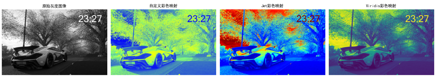
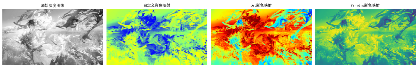
效果说明
- 自定义映射:可根据业务需求设计颜色渐变规则
- Jet映射:经典伪彩色映射,从蓝到红渐变,适合科学可视化
- Viridis映射:Matplotlib默认映射,视觉均匀,适合色盲友好型显示
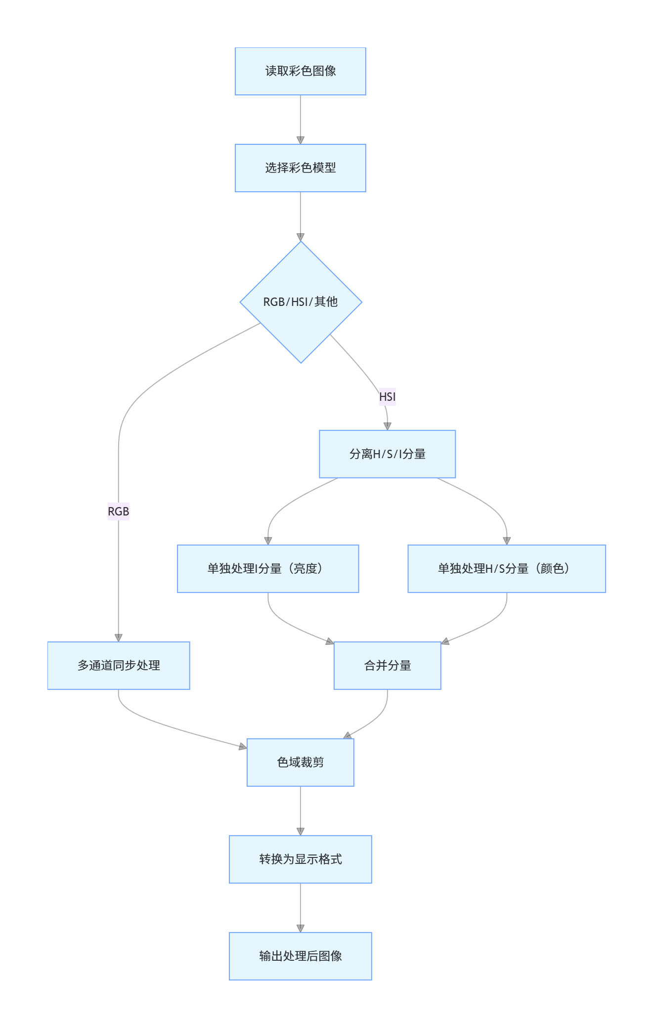
6.4 全彩色图像处理基础
全彩色图像处理直接对RGB/HSI等彩色图像的所有通道进行处理,核心原则:
- 保持颜色一致性:避免单通道处理导致颜色失真
- 亮度与色度分离:HSI模型中I分量处理亮度,H/S分量处理颜色
- 色域约束:处理后像素值需在有效范围(0~255)
代码实现:全彩色图像的基础操作
import cv2
import numpy as np
import matplotlib.pyplot as plt

plt.rcParams['font.sans-serif'] = ['SimHei']
plt.rcParams['axes.unicode_minus'] = False

# 全彩色图像亮度调整
def adjust_brightness(img_rgb, factor):
    # 转换为HSI
    hsi_img, h, s, i = rgb_to_hsi(img_rgb)
    # 调整亮度
    i_adjusted = np.clip(i * factor, 0, 1)
    # 合并HSI
    hsi_adjusted = np.stack([h, s, i_adjusted], axis=-1)
    # 转回RGB
    rgb_adjusted = hsi_to_rgb(hsi_adjusted)
    return rgb_adjusted

# 全彩色图像对比度调整
def adjust_contrast(img_rgb, factor):
    # 转换为浮点数
    img_float = img_rgb.astype(np.float32)
    # 计算均值
    mean = np.mean(img_float, axis=(0, 1), keepdims=True)
    # 调整对比度
    img_contrast = (img_float - mean) * factor + mean
    # 裁剪
    img_contrast = np.clip(img_contrast, 0, 255).astype(np.uint8)
    return img_contrast

# 复用之前的RGB-HSI转换函数
def rgb_to_hsi(img_rgb):
    r = img_rgb[:, :, 0] / 255.0
    g = img_rgb[:, :, 1] / 255.0
    b = img_rgb[:, :, 2] / 255.0
    i = (r + g + b) / 3.0
    min_rgb = np.min(np.stack([r, g, b], axis=-1), axis=-1)
    s = 1 - 3 * min_rgb / (r + g + b + 1e-6)
    s = np.where(r + g + b == 0, 0, s)
    num = 0.5 * ((r - g) + (r - b))
    den = np.sqrt((r - g)**2 + (r - b)*(g - b)) + 1e-6
    theta = np.arccos(num / den)
    h = np.where(b > g, 2 * np.pi - theta, theta)
    h = h / (2 * np.pi)
    hsi_img = np.stack([h, s, i], axis=-1)
    return hsi_img, h, s, i

def hsi_to_rgb(hsi_img):
    h = hsi_img[:, :, 0] * 2 * np.pi
    s = hsi_img[:, :, 1]
    i = hsi_img[:, :, 2]
    r, g, b = np.zeros_like(h), np.zeros_like(h), np.zeros_like(h)
    mask1 = (h >= 0) & (h < 2 * np.pi / 3)
    h1 = h[mask1]
    s1 = s[mask1]
    i1 = i[mask1]
    b1 = i1 * (1 - s1)
    r1 = i1 * (1 + s1 * np.cos(h1) / np.cos(np.pi/3 - h1))
    g1 = 3 * i1 - (r1 + b1)
    r[mask1] = r1
    g[mask1] = g1
    b[mask1] = b1
    mask2 = (h >= 2 * np.pi / 3) & (h < 4 * np.pi / 3)
    h2 = h[mask2] - 2 * np.pi / 3
    s2 = s[mask2]
    i2 = i[mask2]
    r2 = i2 * (1 - s2)
    g2 = i2 * (1 + s2 * np.cos(h2) / np.cos(np.pi/3 - h2))
    b2 = 3 * i2 - (r2 + g2)
    r[mask2] = r2
    g[mask2] = g2
    b[mask2] = b2
    mask3 = (h >= 4 * np.pi / 3) & (h < 2 * np.pi)
    h3 = h[mask3] - 4 * np.pi / 3
    s3 = s[mask3]
    i3 = i[mask3]
    g3 = i3 * (1 - s3)
    b3 = i3 * (1 + s3 * np.cos(h3) / np.cos(np.pi/3 - h3))
    r3 = 3 * i3 - (g3 + b3)
    r[mask3] = r3
    g[mask3] = g3
    b[mask3] = b3
    rgb_img = np.stack([r, g, b], axis=-1)
    rgb_img = np.clip(rgb_img, 0, 1) * 255
    rgb_img = rgb_img.astype(np.uint8)
    return rgb_img

# 主执行
if __name__ == "__main__":
    # 读取图像
    img_path = "test.jpg"
    img_bgr = cv2.imread(img_path)
    img_rgb = cv2.cvtColor(img_bgr, cv2.COLOR_BGR2RGB)

    # 调整亮度(增亮1.5倍)
    img_bright = adjust_brightness(img_rgb, 1.5)
    # 调整亮度(调暗0.5倍)
    img_dark = adjust_brightness(img_rgb, 0.5)
    # 调整对比度(增强2倍)
    img_contrast = adjust_contrast(img_rgb, 2.0)

    # 可视化
    plt.figure(figsize=(18, 6))

    plt.subplot(1, 4, 1)
    plt.imshow(img_rgb)
    plt.title('原始图像')
    plt.axis('off')

    plt.subplot(1, 4, 2)
    plt.imshow(img_bright)
    plt.title('亮度×1.5')
    plt.axis('off')

    plt.subplot(1, 4, 3)
    plt.imshow(img_dark)
    plt.title('亮度×0.5')
    plt.axis('off')

    plt.subplot(1, 4, 4)
    plt.imshow(img_contrast)
    plt.title('对比度×2.0')
    plt.axis('off')

    plt.tight_layout()
    plt.show()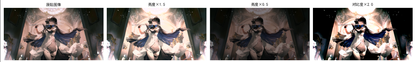
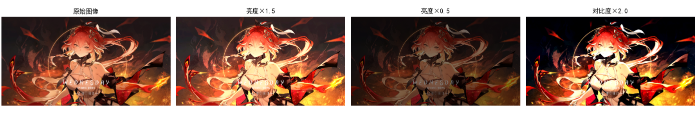
效果说明
- 亮度调整:基于HSI的I分量处理,颜色无失真,仅亮度变化
- 对比度调整:RGB通道同步调整,保持颜色比例,增强细节对比
6.5 彩色变换
彩色变换是对彩色图像的像素值进行数学变换,实现颜色调整、增强等效果。
6.5.1 公式
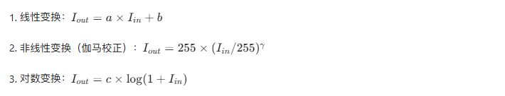
6.5.2 补色
补色是指两种颜色混合后生成白色/灰色,RGB中补色计算:Complement=255−Iin
代码实现:彩色变换(线性+伽马+补色)
import cv2
import numpy as np
import matplotlib.pyplot as plt
plt.rcParams['font.sans-serif'] = ['SimHei']
plt.rcParams['axes.unicode_minus'] = False
# 线性变换
def linear_transform(img_rgb, a=1.0, b=0):
img_float = img_rgb.astype(np.float32)
img_out = a * img_float + b
img_out = np.clip(img_out, 0, 255).astype(np.uint8)
return img_out
# 伽马校正
def gamma_correction(img_rgb, gamma=1.0):
# 构建伽马查找表
gamma_table = np.array([((i / 255.0) ** (1/gamma)) * 255
for i in np.arange(0, 256)]).astype(np.uint8)
# 应用查找表
img_out = cv2.LUT(img_rgb, gamma_table)
return img_out
# 补色变换
def complement_color(img_rgb):
img_complement = 255 - img_rgb
return img_complement
# 对数变换
def log_transform(img_rgb, c=1.0):
img_float = img_rgb.astype(np.float32) + 1 # 避免log(0)
img_out = c * np.log(img_float)
# 归一化到0-255
img_out = (img_out / np.max(img_out)) * 255
img_out = img_out.astype(np.uint8)
return img_out
# 主执行
if __name__ == "__main__":
# 读取图像
img_path = "test.jpg"
img_bgr = cv2.imread(img_path)
img_rgb = cv2.cvtColor(img_bgr, cv2.COLOR_BGR2RGB)
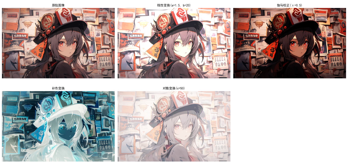
# 线性变换(a=1.5, b=20)
img_linear = linear_transform(img_rgb, 1.5, 20)
# 伽马校正(gamma=0.5)
img_gamma = gamma_correction(img_rgb, 0.5)
# 补色
img_complement = complement_color(img_rgb)
# 对数变换
img_log = log_transform(img_rgb, 50)
# 可视化
plt.figure(figsize=(18, 9))
plt.subplot(2, 3, 1)
plt.imshow(img_rgb)
plt.title('原始图像')
plt.axis('off')
plt.subplot(2, 3, 2)
plt.imshow(img_linear)
plt.title('线性变换(a=1.5, b=20)')
plt.axis('off')
plt.subplot(2, 3, 3)
plt.imshow(img_gamma)
plt.title('伽马校正(γ=0.5)')
plt.axis('off')
plt.subplot(2, 3, 4)
plt.imshow(img_complement)
plt.title('补色变换')
plt.axis('off')
plt.subplot(2, 3, 5)
plt.imshow(img_log)
plt.title('对数变换(c=50)')
plt.axis('off')
plt.tight_layout()
plt.show()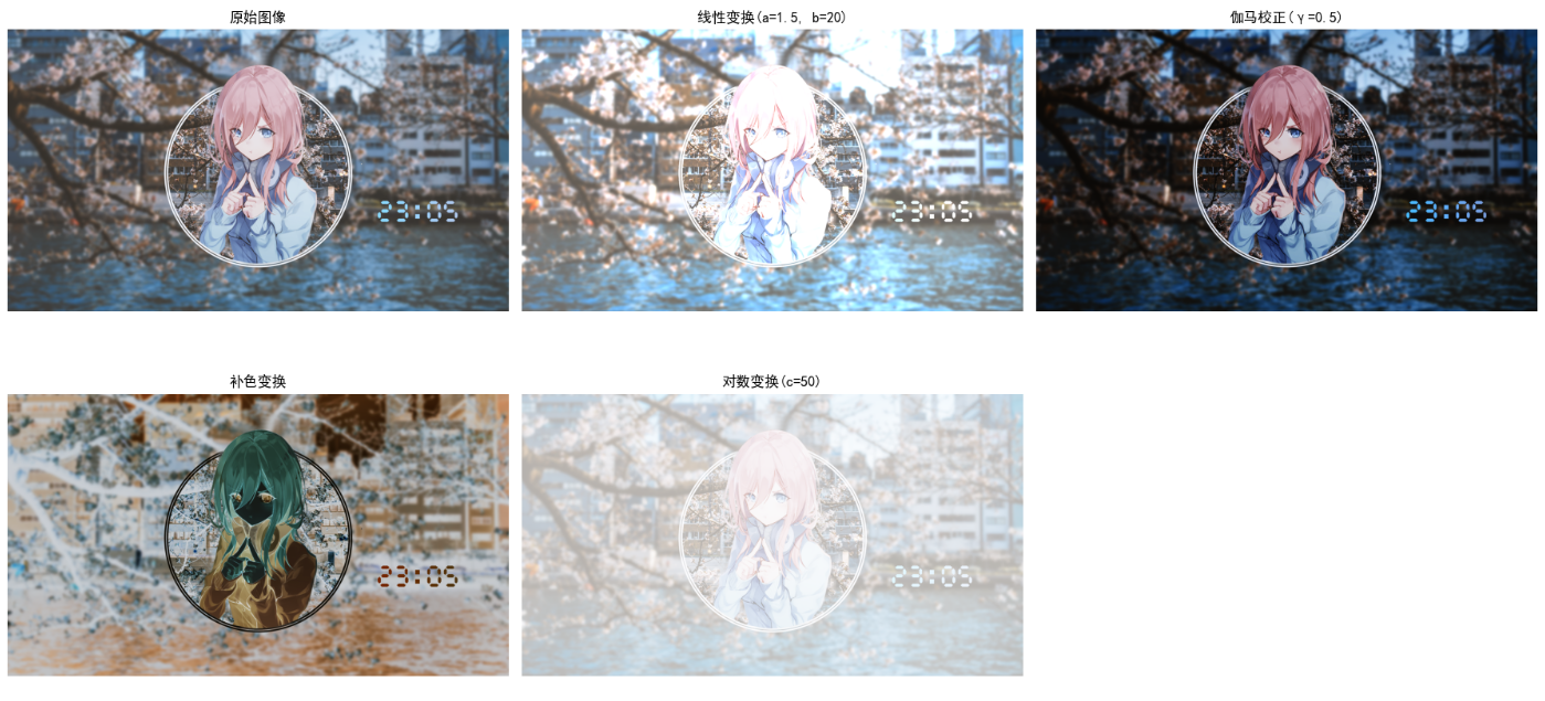
效果说明
- 线性变换:a>1增强对比度,b>0提升亮度
- 伽马校正:γ<1提亮图像,γ>1调暗图像,适合校正显示器亮度
- 补色变换:生成反色图像,如红→青、绿→品红、蓝→黄
- 对数变换:压缩高光,增强暗部细节
6.5.3 彩色分层
彩色分层是对RGB/HSI的特定通道进行分层处理,提取目标颜色区域。
代码实现:HSI彩色分层提取红色区域
import cv2
import numpy as np
import matplotlib.pyplot as plt

plt.rcParams['font.sans-serif'] = ['SimHei']
plt.rcParams['axes.unicode_minus'] = False

# HSI彩色分层
def hsi_color_layer(img_rgb, h_range=(0, 30), s_range=(0.5, 1.0), i_range=(0.2, 1.0)):
    # 转HSI
    hsi_img, h, s, i = rgb_to_hsi(img_rgb)

    # 转换H范围(0-360°)
    h_deg = h * 360

    # 创建掩码
    mask_h = (h_deg >= h_range[0]) | (h_deg <= 360 + h_range[1])  # 红色跨0°/360°
    mask_s = (s >= s_range[0]) & (s <= s_range[1])
    mask_i = (i >= i_range[0]) & (i <= i_range[1])
    mask = mask_h & mask_s & mask_i

    # 提取目标区域
    color_layer = np.zeros_like(img_rgb)
    color_layer[mask] = img_rgb[mask]

    # 掩码可视化
    mask_vis = mask.astype(np.uint8) * 255

    return color_layer, mask_vis

# 复用RGB-HSI转换函数
def rgb_to_hsi(img_rgb):
    r = img_rgb[:, :, 0] / 255.0
    g = img_rgb[:, :, 1] / 255.0
    b = img_rgb[:, :, 2] / 255.0
    i = (r + g + b) / 3.0
    min_rgb = np.min(np.stack([r, g, b], axis=-1), axis=-1)
    s = 1 - 3 * min_rgb / (r + g + b + 1e-6)
    s = np.where(r + g + b == 0, 0, s)
    num = 0.5 * ((r - g) + (r - b))
    den = np.sqrt((r - g)**2 + (r - b)*(g - b)) + 1e-6
    theta = np.arccos(num / den)
    h = np.where(b > g, 2 * np.pi - theta, theta)
    h = h / (2 * np.pi)
    hsi_img = np.stack([h, s, i], axis=-1)
    return hsi_img, h, s, i

# 主执行
if __name__ == "__main__":
    # 读取包含红色物体的图像
    img_path = "red_object.jpg"  # 建议使用含红色物体的图像
    try:
        img_bgr = cv2.imread(img_path)
        img_rgb = cv2.cvtColor(img_bgr, cv2.COLOR_BGR2RGB)
    except:
        # 生成测试图像
        img_rgb = np.zeros((400, 400, 3), dtype=np.uint8)
        # 绘制红色圆形
        cv2.circle(img_rgb, (200, 200), 100, (255, 0, 0), -1)

    # 提取红色区域(H:0-30°, S:0.5-1.0, I:0.2-1.0)
    red_layer, mask_vis = hsi_color_layer(img_rgb)

    # 可视化
    plt.figure(figsize=(15, 5))

    plt.subplot(1, 3, 1)
    plt.imshow(img_rgb)
    plt.title('原始图像')
    plt.axis('off')

    plt.subplot(1, 3, 2)
    plt.imshow(mask_vis, cmap='gray')
    plt.title('红色区域掩码')
    plt.axis('off')

    plt.subplot(1, 3, 3)
    plt.imshow(red_layer)
    plt.title('提取的红色区域')
    plt.axis('off')

    plt.tight_layout()
    plt.show()
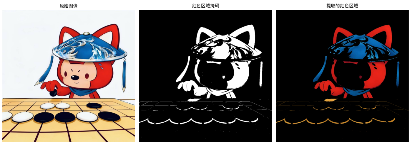
效果说明
- 掩码图:白色区域为提取的红色区域,黑色为背景
- 提取结果:仅保留红色区域,背景置黑,实现颜色分层提取
6.5.4 色调和彩色校正
彩色校正用于修正图像的颜色偏差(如白平衡),常用灰度世界法、完美反射法。
代码实现:灰度世界法白平衡校正
import cv2
import numpy as np
import matplotlib.pyplot as plt

plt.rcParams['font.sans-serif'] = ['SimHei']
plt.rcParams['axes.unicode_minus'] = False

# 灰度世界法白平衡
def gray_world_white_balance(img_rgb):
    # 计算各通道均值
    r_mean = np.mean(img_rgb[:, :, 0])
    g_mean = np.mean(img_rgb[:, :, 1])
    b_mean = np.mean(img_rgb[:, :, 2])

    # 计算增益
    gray_mean = (r_mean + g_mean + b_mean) / 3
    r_gain = gray_mean / r_mean
    g_gain = gray_mean / g_mean
    b_gain = gray_mean / b_mean

    # 应用增益
    img_corrected = img_rgb.astype(np.float32)
    img_corrected[:, :, 0] *= r_gain
    img_corrected[:, :, 1] *= g_gain
    img_corrected[:, :, 2] *= b_gain

    # 裁剪
    img_corrected = np.clip(img_corrected, 0, 255).astype(np.uint8)
    return img_corrected

# 完美反射法白平衡
def perfect_reflect_white_balance(img_rgb, percentile=95):
    # 计算各通道百分位值
    r_percent = np.percentile(img_rgb[:, :, 0], percentile)
    g_percent = np.percentile(img_rgb[:, :, 1], percentile)
    b_percent = np.percentile(img_rgb[:, :, 2], percentile)

    # 计算增益
    r_gain = 255 / r_percent
    g_gain = 255 / g_percent
    b_gain = 255 / b_percent

    # 应用增益
    img_corrected = img_rgb.astype(np.float32)
    img_corrected[:, :, 0] *= r_gain
    img_corrected[:, :, 1] *= g_gain
    img_corrected[:, :, 2] *= b_gain

    # 裁剪
    img_corrected = np.clip(img_corrected, 0, 255).astype(np.uint8)
    return img_corrected

# 主执行
if __name__ == "__main__":
    # 读取偏色图像(如偏黄/偏蓝的室内照片)
    img_path = "color_cast.jpg"
    try:
        img_bgr = cv2.imread(img_path)
        img_rgb = cv2.cvtColor(img_bgr, cv2.COLOR_BGR2RGB)
    except:
        # 生成偏色测试图像
        img_rgb = cv2.imread("test.jpg")
        img_rgb = cv2.cvtColor(img_rgb, cv2.COLOR_BGR2RGB)
        # 模拟偏黄(增加红、绿通道)
        img_rgb[:, :, 0] = np.clip(img_rgb[:, :, 0] * 1.2, 0, 255).astype(np.uint8)
        img_rgb[:, :, 1] = np.clip(img_rgb[:, :, 1] * 1.2, 0, 255).astype(np.uint8)

    # 灰度世界法校正
    img_gray_world = gray_world_white_balance(img_rgb)
    # 完美反射法校正
    img_perfect = perfect_reflect_white_balance(img_rgb)

    # 可视化
    plt.figure(figsize=(18, 6))

    plt.subplot(1, 3, 1)
    plt.imshow(img_rgb)
    plt.title('偏色原始图像')
    plt.axis('off')

    plt.subplot(1, 3, 2)
    plt.imshow(img_gray_world)
    plt.title('灰度世界法校正')
    plt.axis('off')

    plt.subplot(1, 3, 3)
    plt.imshow(img_perfect)
    plt.title('完美反射法校正')
    plt.axis('off')

    plt.tight_layout()
    plt.show()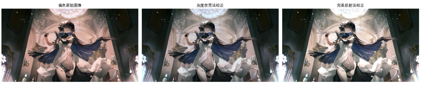
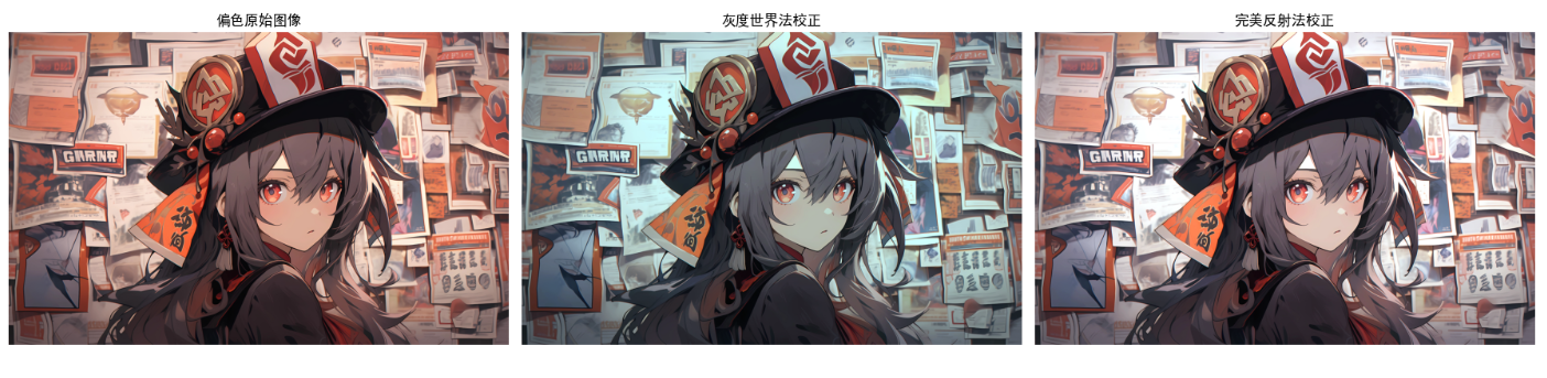
效果说明
- 灰度世界法:假设图像各通道均值相等,适合自然场景图像
- 完美反射法:假设图像中最亮区域为白色,适合有高光的图像
- 校正后图像颜色更接近真实场景,偏色问题得到解决
6.5.5 彩色图像的直方图处理
彩色直方图处理包括单通道直方图均衡化、多通道同步均衡化、HSI的I分量均衡化(保持颜色)。
代码实现:彩色图像直方图处理
import cv2
import numpy as np
import matplotlib.pyplot as plt

plt.rcParams['font.sans-serif'] = ['SimHei']
plt.rcParams['axes.unicode_minus'] = False

# 单通道直方图均衡化(RGB各通道单独均衡)
def rgb_hist_equalize(img_rgb):
    r_eq = cv2.equalizeHist(img_rgb[:, :, 0])
    g_eq = cv2.equalizeHist(img_rgb[:, :, 1])
    b_eq = cv2.equalizeHist(img_rgb[:, :, 2])
    img_eq = np.stack([r_eq, g_eq, b_eq], axis=-1)
    return img_eq

# HSI的I分量均衡化(保持颜色)
def hsi_i_hist_equalize(img_rgb):
    # 转HSI
    hsi_img, h, s, i = rgb_to_hsi(img_rgb)
    # I分量均衡化
    i_eq = cv2.equalizeHist((i * 255).astype(np.uint8)) / 255.0
    # 合并HSI
    hsi_eq = np.stack([h, s, i_eq], axis=-1)
    # 转回RGB
    img_eq = hsi_to_rgb(hsi_eq)
    return img_eq

# 计算彩色直方图
def calc_color_hist(img_rgb):
    hist_r = cv2.calcHist([img_rgb], [0], None, [256], [0, 256])
    hist_g = cv2.calcHist([img_rgb], [1], None, [256], [0, 256])
    hist_b = cv2.calcHist([img_rgb], [2], None, [256], [0, 256])
    return hist_r, hist_g, hist_b

# 复用RGB-HSI转换函数
def rgb_to_hsi(img_rgb):
    r = img_rgb[:, :, 0] / 255.0
    g = img_rgb[:, :, 1] / 255.0
    b = img_rgb[:, :, 2] / 255.0
    i = (r + g + b) / 3.0
    min_rgb = np.min(np.stack([r, g, b], axis=-1), axis=-1)
    s = 1 - 3 * min_rgb / (r + g + b + 1e-6)
    s = np.where(r + g + b == 0, 0, s)
    num = 0.5 * ((r - g) + (r - b))
    den = np.sqrt((r - g)**2 + (r - b)*(g - b)) + 1e-6
    theta = np.arccos(num / den)
    h = np.where(b > g, 2 * np.pi - theta, theta)
    h = h / (2 * np.pi)
    hsi_img = np.stack([h, s, i], axis=-1)
    return hsi_img, h, s, i

def hsi_to_rgb(hsi_img):
    h = hsi_img[:, :, 0] * 2 * np.pi
    s = hsi_img[:, :, 1]
    i = hsi_img[:, :, 2]
    r, g, b = np.zeros_like(h), np.zeros_like(h), np.zeros_like(h)
    mask1 = (h >= 0) & (h < 2 * np.pi / 3)
    h1 = h[mask1]
    s1 = s[mask1]
    i1 = i[mask1]
    b1 = i1 * (1 - s1)
    r1 = i1 * (1 + s1 * np.cos(h1) / np.cos(np.pi/3 - h1))
    g1 = 3 * i1 - (r1 + b1)
    r[mask1] = r1
    g[mask1] = g1
    b[mask1] = b1
    mask2 = (h >= 2 * np.pi / 3) & (h < 4 * np.pi / 3)
    h2 = h[mask2] - 2 * np.pi / 3
    s2 = s[mask2]
    i2 = i[mask2]
    r2 = i2 * (1 - s2)
    g2 = i2 * (1 + s2 * np.cos(h2) / np.cos(np.pi/3 - h2))
    b2 = 3 * i2 - (r2 + g2)
    r[mask2] = r2
    g[mask2] = g2
    b[mask2] = b2
    mask3 = (h >= 4 * np.pi / 3) & (h < 2 * np.pi)
    h3 = h[mask3] - 4 * np.pi / 3
    s3 = s[mask3]
    i3 = i[mask3]
    g3 = i3 * (1 - s3)
    b3 = i3 * (1 + s3 * np.cos(h3) / np.cos(np.pi/3 - h3))
    r3 = 3 * i3 - (g3 + b3)
    r[mask3] = r3
    g[mask3] = g3
    b[mask3] = b3
    rgb_img = np.stack([r, g, b], axis=-1)
    rgb_img = np.clip(rgb_img, 0, 1) * 255
    rgb_img = rgb_img.astype(np.uint8)
    return rgb_img

# 主执行
if __name__ == "__main__":
    # 读取低对比度彩色图像
    img_path = "low_contrast.jpg"
    try:
        img_bgr = cv2.imread(img_path)
        img_rgb = cv2.cvtColor(img_bgr, cv2.COLOR_BGR2RGB)
    except:
        # 生成低对比度测试图像
        img_rgb = cv2.imread("test.jpg")
        img_rgb = cv2.cvtColor(img_rgb, cv2.COLOR_BGR2RGB)
        img_rgb = (img_rgb * 0.5 + 50).astype(np.uint8)  # 降低对比度

    # RGB各通道均衡化
    img_rgb_eq = rgb_hist_equalize(img_rgb)
    # HSI的I分量均衡化
    img_hsi_eq = hsi_i_hist_equalize(img_rgb)

    # 计算直方图
    hist_r, hist_g, hist_b = calc_color_hist(img_rgb)
    hist_r_eq, hist_g_eq, hist_b_eq = calc_color_hist(img_rgb_eq)
    hist_r_hsi, hist_g_hsi, hist_b_hsi = calc_color_hist(img_hsi_eq)

    # 可视化图像
    plt.figure(figsize=(18, 6))
    plt.subplot(1, 3, 1)
    plt.imshow(img_rgb)
    plt.title('原始低对比度图像')
    plt.axis('off')

    plt.subplot(1, 3, 2)
    plt.imshow(img_rgb_eq)
    plt.title('RGB各通道均衡化(颜色失真)')
    plt.axis('off')

    plt.subplot(1, 3, 3)
    plt.imshow(img_hsi_eq)
    plt.title('HSI-I分量均衡化(颜色保持)')
    plt.axis('off')
    plt.show()

    # 可视化直方图
    plt.figure(figsize=(18, 12))

    # 原始直方图
    plt.subplot(3, 1, 1)
    plt.plot(hist_r, color='r', label='R通道')
    plt.plot(hist_g, color='g', label='G通道')
    plt.plot(hist_b, color='b', label='B通道')
    plt.title('原始图像直方图')
    plt.legend()
    plt.xlim([0, 256])

    # RGB均衡化直方图
    plt.subplot(3, 1, 2)
    plt.plot(hist_r_eq, color='r', label='R通道')
    plt.plot(hist_g_eq, color='g', label='G通道')
    plt.plot(hist_b_eq, color='b', label='B通道')
    plt.title('RGB均衡化直方图')
    plt.legend()
    plt.xlim([0, 256])

    # HSI均衡化直方图
    plt.subplot(3, 1, 3)
    plt.plot(hist_r_hsi, color='r', label='R通道')
    plt.plot(hist_g_hsi, color='g', label='G通道')
    plt.plot(hist_b_hsi, color='b', label='B通道')
    plt.title('HSI-I均衡化直方图')
    plt.legend()
    plt.xlim([0, 256])

    plt.tight_layout()
    plt.show()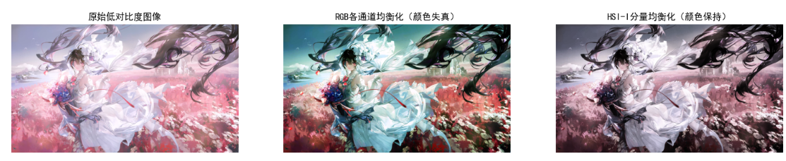
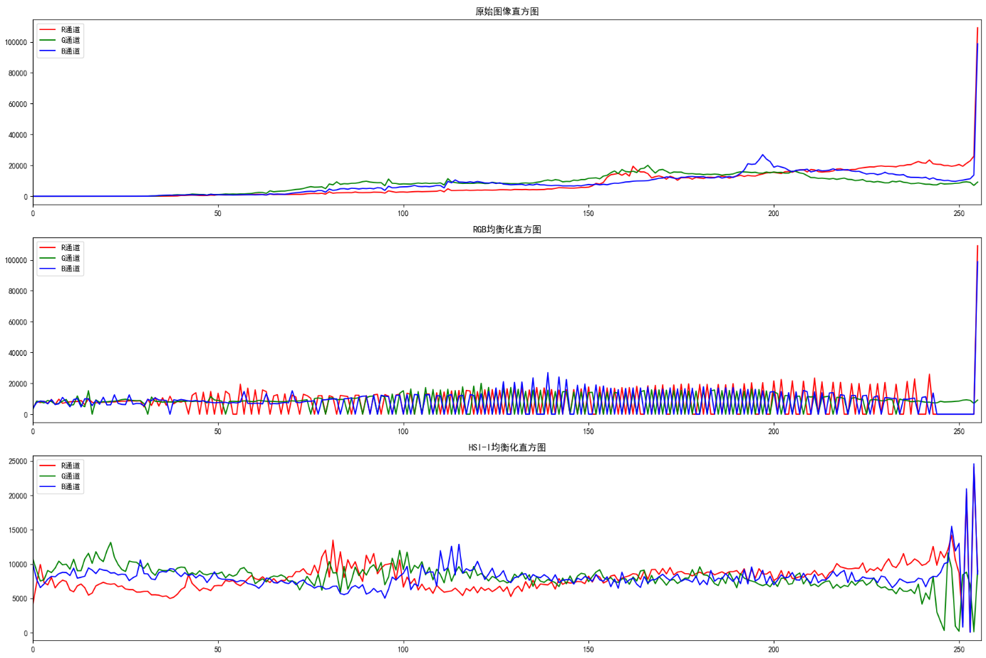
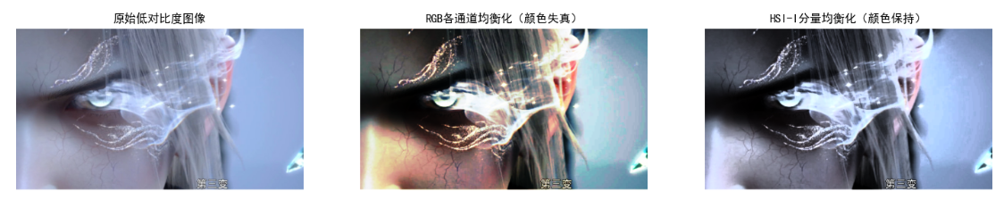
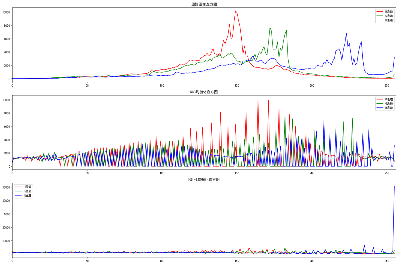
效果说明
- RGB各通道均衡化:对比度提升,但颜色失真(如偏色)
- HSI-I分量均衡化:对比度提升,且颜色保持自然(推荐使用)
- 直方图:均衡化后直方图分布更均匀,暗部/亮部细节更丰富
6.6 彩色图像平滑和锐化
彩色图像的平滑与锐化是增强图像质量的核心操作,需遵循「多通道同步处理」原则,避免单通道操作导致颜色失真。
6.6.1 彩色图像平滑
彩色图像平滑的目标是降低噪声、模糊细节,常用方法包括高斯滤波 (平滑高斯噪声)、中值滤波 (抑制椒盐噪声)、双边滤波(保边平滑)。
核心原理
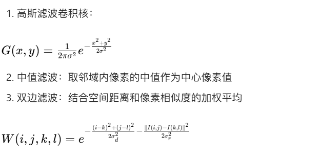
代码实现:彩色图像平滑(对比不同滤波效果)
import cv2
import numpy as np
import matplotlib.pyplot as plt

# 设置中文显示
plt.rcParams['font.sans-serif'] = ['SimHei']
plt.rcParams['axes.unicode_minus'] = False

# 1. 生成含噪声的彩色图像
def add_noise_to_color(img_rgb, noise_type="gaussian"):
    """
    给彩色图像添加噪声
    :param img_rgb: RGB格式图像
    :param noise_type: 噪声类型(gaussian/ salt_pepper)
    :return: 含噪声图像
    """
    img_float = img_rgb.astype(np.float32)
    h, w, c = img_rgb.shape

    if noise_type == "gaussian":
        # 高斯噪声(均值0,标准差20)
        noise = np.random.normal(0, 20, (h, w, c))
        img_noisy = img_float + noise
    elif noise_type == "salt_pepper":
        # 椒盐噪声(5%噪声密度)
        img_noisy = img_float.copy()
        mask = np.random.choice([0, 1, 2], size=(h, w), p=[0.025, 0.025, 0.95])
        img_noisy[mask == 0] = 0    # 椒噪声(黑)
        img_noisy[mask == 1] = 255  # 盐噪声(白)
    else:
        return img_rgb

    # 裁剪到0-255范围
    img_noisy = np.clip(img_noisy, 0, 255).astype(np.uint8)
    return img_noisy

# 2. 彩色图像平滑处理
def color_image_smoothing(img_noisy):
    """
    彩色图像平滑(高斯/中值/双边滤波)
    :param img_noisy: 含噪声图像
    :return: 各类滤波结果
    """
    # 高斯滤波(5x5核,σ=1.5)
    gaussian_blur = cv2.GaussianBlur(img_noisy, (5, 5), 1.5)
    # 中值滤波(5x5核)
    median_blur = cv2.medianBlur(img_noisy, 5)
    # 双边滤波(直径9,空间σ=75,灰度σ=75)
    bilateral_blur = cv2.bilateralFilter(img_noisy, 9, 75, 75)

    return gaussian_blur, median_blur, bilateral_blur

# 3. 主执行逻辑
if __name__ == "__main__":
    # 读取测试图像(替换为自己的图像路径)
    img_bgr = cv2.imread("test.jpg")
    img_rgb = cv2.cvtColor(img_bgr, cv2.COLOR_BGR2RGB)

    # 生成含噪声图像(分别测试高斯/椒盐噪声)
    img_gaussian_noise = add_noise_to_color(img_rgb, "gaussian")
    img_sp_noise = add_noise_to_color(img_rgb, "salt_pepper")

    # 对高斯噪声图像平滑
    gauss_smooth, median_smooth, bilateral_smooth = color_image_smoothing(img_gaussian_noise)

    # 可视化结果(高斯噪声+平滑)
    plt.figure(figsize=(18, 10))
    plt.subplot(2, 3, 1)
    plt.imshow(img_rgb)
    plt.title("原始RGB图像")
    plt.axis("off")

    plt.subplot(2, 3, 2)
    plt.imshow(img_gaussian_noise)
    plt.title("添加高斯噪声后")
    plt.axis("off")

    plt.subplot(2, 3, 3)
    plt.imshow(gauss_smooth)
    plt.title("高斯滤波(5x5)")
    plt.axis("off")

    plt.subplot(2, 3, 4)
    plt.imshow(median_smooth)
    plt.title("中值滤波(5x5)")
    plt.axis("off")

    plt.subplot(2, 3, 5)
    plt.imshow(bilateral_smooth)
    plt.title("双边滤波(保边平滑)")
    plt.axis("off")
    plt.show()

    # 对椒盐噪声图像平滑(重点看中值滤波效果)
    sp_gauss, sp_median, sp_bilateral = color_image_smoothing(img_sp_noise)
    plt.figure(figsize=(18, 6))
    plt.subplot(1, 4, 1)
    plt.imshow(img_sp_noise)
    plt.title("添加椒盐噪声后")
    plt.axis("off")

    plt.subplot(1, 4, 2)
    plt.imshow(sp_gauss)
    plt.title("高斯滤波(效果差)")
    plt.axis("off")

    plt.subplot(1, 4, 3)
    plt.imshow(sp_median)
    plt.title("中值滤波(效果好)")
    plt.axis("off")

    plt.subplot(1, 4, 4)
    plt.imshow(sp_bilateral)
    plt.title("双边滤波(中等效果)")
    plt.axis("off")
    plt.show()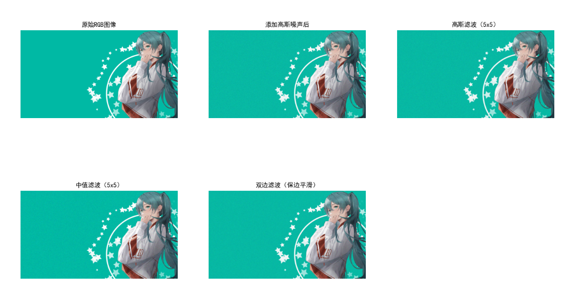

效果说明
- 高斯噪声:高斯滤波、双边滤波效果最优,中值滤波次之;
- 椒盐噪声:中值滤波几乎可完全消除噪声,高斯滤波仅能模糊噪声(效果差);
- 双边滤波:在平滑噪声的同时保留图像边缘(如物体轮廓),是「保边平滑」的首选。
6.6.2 彩色图像锐化
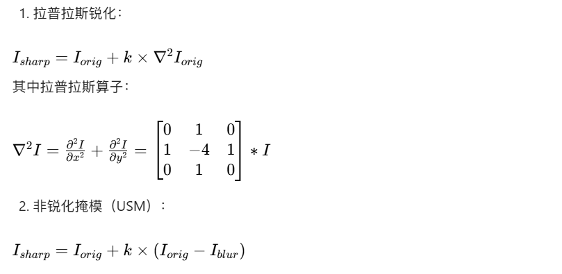
彩色图像锐化的目标是增强边缘和细节,核心思路是「原图 - 平滑图 = 边缘图」,再将边缘图叠加回原图。
核心原理
代码实现:彩色图像锐化(拉普拉斯 + USM)
import cv2
import numpy as np
import matplotlib.pyplot as plt

plt.rcParams['font.sans-serif'] = ['SimHei']
plt.rcParams['axes.unicode_minus'] = False

# 1. 拉普拉斯锐化
def laplacian_sharpening(img_rgb, k=1.0):
    """
    彩色图像拉普拉斯锐化
    :param img_rgb: RGB图像
    :param k: 锐化强度系数
    :return: 锐化后图像
    """
    # 定义拉普拉斯算子(3x3)
    laplacian_kernel = np.array([[0, 1, 0],
                                 [1, -4, 1],
                                 [0, 1, 0]], dtype=np.float32)

    # 对每个通道单独锐化(避免颜色失真)
    sharp_channels = []
    for c in range(3):
        channel = img_rgb[:, :, c].astype(np.float32)
        # 卷积计算拉普拉斯边缘
        laplacian = cv2.filter2D(channel, -1, laplacian_kernel)
        # 锐化公式:原图 + k*边缘
        sharp_channel = channel + k * laplacian
        # 裁剪范围
        sharp_channel = np.clip(sharp_channel, 0, 255).astype(np.uint8)
        sharp_channels.append(sharp_channel)

    # 合并通道
    img_sharp = np.stack(sharp_channels, axis=-1)
    return img_sharp

# 2. USM锐化(非锐化掩模)
def usm_sharpening(img_rgb, blur_size=(5,5), sigma=1.5, k=1.5):
    """
    彩色图像USM锐化
    :param img_rgb: RGB图像
    :param blur_size: 高斯模糊核大小
    :param sigma: 高斯模糊标准差
    :param k: 锐化强度
    :return: 锐化后图像
    """
    # 高斯模糊生成模糊图
    img_blur = cv2.GaussianBlur(img_rgb, blur_size, sigma)
    # 计算边缘图(原图 - 模糊图)
    img_edge = img_rgb.astype(np.float32) - img_blur.astype(np.float32)
    # 锐化:原图 + k*边缘
    img_sharp = img_rgb.astype(np.float32) + k * img_edge
    # 裁剪范围
    img_sharp = np.clip(img_sharp, 0, 255).astype(np.uint8)
    return img_sharp

# 3. 主执行逻辑
if __name__ == "__main__":
    # 读取图像
    img_bgr = cv2.imread("test.jpg")
    img_rgb = cv2.cvtColor(img_bgr, cv2.COLOR_BGR2RGB)

    # 拉普拉斯锐化(k=1.0)
    laplacian_sharp = laplacian_sharpening(img_rgb, k=1.0)
    # USM锐化(k=1.5)
    usm_sharp = usm_sharpening(img_rgb, k=1.5)

    # 可视化对比
    plt.figure(figsize=(18, 6))
    plt.subplot(1, 3, 1)
    plt.imshow(img_rgb)
    plt.title("原始RGB图像")
    plt.axis("off")

    plt.subplot(1, 3, 2)
    plt.imshow(laplacian_sharp)
    plt.title("拉普拉斯锐化(k=1.0)")
    plt.axis("off")

    plt.subplot(1, 3, 3)
    plt.imshow(usm_sharp)
    plt.title("USM锐化(k=1.5)")
    plt.axis("off")
    plt.show()

    # 锐化强度对比(USM不同k值)
    usm_k05 = usm_sharpening(img_rgb, k=0.5)
    usm_k20 = usm_sharpening(img_rgb, k=2.0)
    plt.figure(figsize=(18, 6))
    plt.subplot(1, 3, 1)
    plt.imshow(usm_k05)
    plt.title("USM锐化(k=0.5,弱)")
    plt.axis("off")

    plt.subplot(1, 3, 2)
    plt.imshow(usm_sharp)
    plt.title("USM锐化(k=1.5,中)")
    plt.axis("off")

    plt.subplot(1, 3, 3)
    plt.imshow(usm_k20)
    plt.title("USM锐化(k=2.0,强)")
    plt.axis("off")
    plt.show()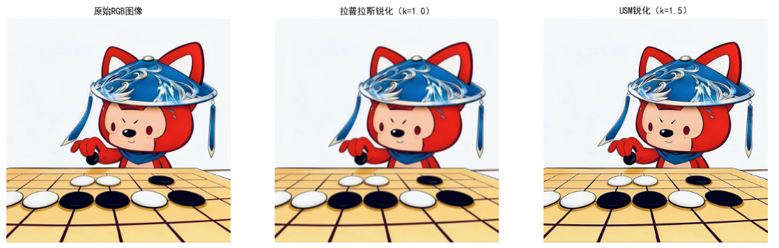
效果说明
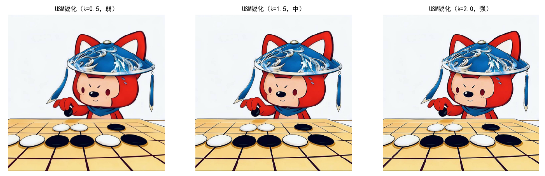
- 拉普拉斯锐化:增强高频细节(如纹理),但易放大噪声;
- USM 锐化:效果更自然,是 Photoshop 等软件的默认锐化方式;
- 锐化强度 k:k 越大锐化越明显,但 k 过大会导致图像失真、出现伪影。
6.7 使用彩色分割图像
彩色分割是根据颜色特征将图像划分为不同区域,核心优势是比灰度分割更精准(利用颜色维度信息)。
6.7.1 HSI 彩色空间中的分割
HSI 空间更贴合人类视觉感知,色调(H) 是分割的核心特征(不受亮度影响),适合分割特定颜色的物体(如红色苹果、绿色树叶)。
代码实现:HSI 空间分割红色区域
import cv2
import numpy as np
import matplotlib.pyplot as plt

plt.rcParams['font.sans-serif'] = ['SimHei']
plt.rcParams['axes.unicode_minus'] = False

# 1. RGB转HSI(复用之前的函数,补充完整)
def rgb_to_hsi(img_rgb):
    """
    RGB转HSI(归一化到[0,1])
    :param img_rgb: RGB图像(0-255)
    :return: hsi_img, h, s, i
    """
    # 归一化到0-1
    r = img_rgb[:, :, 0] / 255.0
    g = img_rgb[:, :, 1] / 255.0
    b = img_rgb[:, :, 2] / 255.0

    # 计算亮度I
    i = (r + g + b) / 3.0

    # 计算饱和度S
    min_rgb = np.min(np.stack([r, g, b], axis=-1), axis=-1)
    s = 1 - 3 * min_rgb / (r + g + b + 1e-6)  # 避免除0
    s = np.where(r + g + b == 0, 0, s)  # 黑色区域S=0

    # 计算色调H(弧度转角度,0-360)
    num = 0.5 * ((r - g) + (r - b))
    den = np.sqrt((r - g)**2 + (r - b)*(g - b)) + 1e-6
    theta = np.arccos(num / den)
    h = np.where(b > g, 2 * np.pi - theta, theta)  # 弧度
    h = h / (2 * np.pi) * 360  # 转换为0-360度

    # 合并HSI
    hsi_img = np.stack([h, s, i], axis=-1)
    return hsi_img, h, s, i

# 2. HSI空间颜色分割
def hsi_color_segmentation(img_rgb, h_range, s_range=(0.2, 1.0), i_range=(0.1, 1.0)):
    """
    HSI空间颜色分割
    :param img_rgb: RGB图像
    :param h_range: 色调范围(如红色:(0, 30) 或 (330, 360))
    :param s_range: 饱和度范围
    :param i_range: 亮度范围
    :return: 分割掩码、分割结果图像
    """
    # 转HSI
    hsi_img, h, s, i = rgb_to_hsi(img_rgb)

    # 构建掩码(处理红色跨0度的情况)
    if h_range[0] > h_range[1]:  # 如(330, 360) + (0, 30)
        mask_h = (h >= h_range[0]) | (h <= h_range[1])
    else:
        mask_h = (h >= h_range[0]) & (h <= h_range[1])

    # 饱和度和亮度掩码
    mask_s = (s >= s_range[0]) & (s <= s_range[1])
    mask_i = (i >= i_range[0]) & (i <= i_range[1])

    # 合并掩码
    mask = mask_h & mask_s & mask_i
    mask_uint8 = mask.astype(np.uint8) * 255  # 转换为0-255

    # 应用掩码到原图
    seg_result = np.zeros_like(img_rgb)
    seg_result[mask] = img_rgb[mask]

    return mask_uint8, seg_result

# 3. 主执行逻辑
if __name__ == "__main__":
    # 读取含红色物体的图像(如红苹果、红玫瑰)
    img_bgr = cv2.imread("red_object.jpg")
    img_rgb = cv2.cvtColor(img_bgr, cv2.COLOR_BGR2RGB)

    # 分割红色区域(H: 0-30 或 330-360,S:0.2-1.0,I:0.1-1.0)
    red_mask, red_seg = hsi_color_segmentation(img_rgb, h_range=(330, 30))

    # 可视化结果
    plt.figure(figsize=(18, 6))
    plt.subplot(1, 3, 1)
    plt.imshow(img_rgb)
    plt.title("原始图像")
    plt.axis("off")

    plt.subplot(1, 3, 2)
    plt.imshow(red_mask, cmap="gray")
    plt.title("红色区域掩码")
    plt.axis("off")

    plt.subplot(1, 3, 3)
    plt.imshow(red_seg)
    plt.title("HSI分割结果(仅保留红色)")
    plt.axis("off")
    plt.show()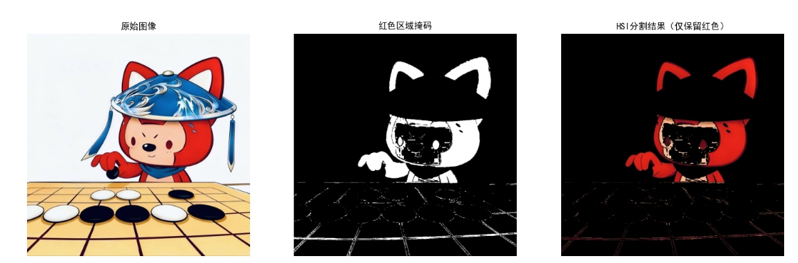
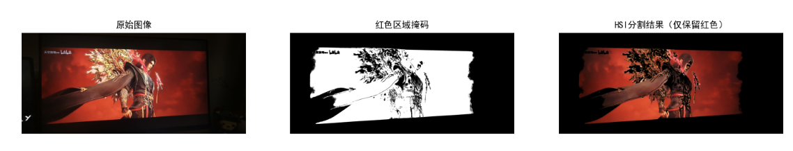
效果说明
- 掩码图:白色区域为目标颜色(红色),黑色为背景;
- 分割结果:仅保留红色区域,背景置黑,分割精度远高于 RGB 空间;
- 优势:不受光照(亮度 I)影响,即使物体明暗不均也能精准分割。
6.7.2 RGB 空间中的分割
RGB 空间分割直接基于三通道像素值阈值,适合颜色特征单一、光照均匀的场景(如纯色物体分割)。
代码实现:RGB 空间分割绿色植物
import cv2
import numpy as np
import matplotlib.pyplot as plt

plt.rcParams['font.sans-serif'] = ['SimHei']
plt.rcParams['axes.unicode_minus'] = False

# RGB颜色分割
def rgb_color_segmentation(img_rgb, r_range, g_range, b_range):
    """
    RGB空间颜色分割
    :param img_rgb: RGB图像
    :param r_range: R通道阈值范围
    :param g_range: G通道阈值范围
    :param b_range: B通道阈值范围
    :return: 掩码、分割结果
    """
    # 提取各通道
    r = img_rgb[:, :, 0]
    g = img_rgb[:, :, 1]
    b = img_rgb[:, :, 2]

    # 构建各通道掩码
    mask_r = (r >= r_range[0]) & (r <= r_range[1])
    mask_g = (g >= g_range[0]) & (g <= g_range[1])
    mask_b = (b >= b_range[0]) & (b <= b_range[1])

    # 合并掩码
    mask = mask_r & mask_g & mask_b
    mask_uint8 = mask.astype(np.uint8) * 255

    # 分割结果
    seg_result = np.zeros_like(img_rgb)
    seg_result[mask] = img_rgb[mask]

    return mask_uint8, seg_result

# 主执行逻辑
if __name__ == "__main__":
    # 读取含绿色植物的图像
    img_bgr = cv2.imread("green_plant.jpg")
    img_rgb = cv2.cvtColor(img_bgr, cv2.COLOR_BGR2RGB)

    # 分割绿色区域(R:0-100, G:50-255, B:0-100)
    green_mask, green_seg = rgb_color_segmentation(
        img_rgb,
        r_range=(0, 100),
        g_range=(50, 255),
        b_range=(0, 100)
    )

    # 可视化
    plt.figure(figsize=(18, 6))
    plt.subplot(1, 3, 1)
    plt.imshow(img_rgb)
    plt.title("原始图像")
    plt.axis("off")

    plt.subplot(1, 3, 2)
    plt.imshow(green_mask, cmap="gray")
    plt.title("绿色区域掩码")
    plt.axis("off")

    plt.subplot(1, 3, 3)
    plt.imshow(green_seg)
    plt.title("RGB分割结果(仅保留绿色)")
    plt.axis("off")
    plt.show()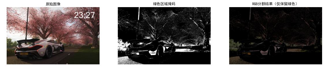
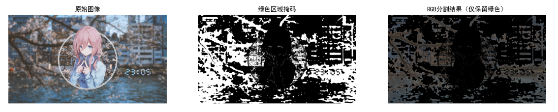
效果说明
- 优势:计算简单、速度快,无需颜色空间转换;
- 劣势:受光照影响大(如强光下绿色会偏白,阈值需调整);
- 适用场景:静态、光照均匀的场景(如工业质检中的纯色零件分割)。
6.7.3 彩色边缘检测
彩色边缘检测结合多通道边缘信息,常用方法包括「RGB 各通道边缘融合」「HSI 的 H/S 通道边缘检测」。
代码实现:彩色边缘检测(Canny + 多通道融合)
import cv2
import numpy as np
import matplotlib.pyplot as plt

plt.rcParams['font.sans-serif'] = ['SimHei']
plt.rcParams['axes.unicode_minus'] = False

# 彩色边缘检测
def color_edge_detection(img_rgb, canny_low=50, canny_high=150):
    """
    彩色边缘检测(两种方法)
    :param img_rgb: RGB图像
    :param canny_low: Canny低阈值
    :param canny_high: Canny高阈值
    :return: 方法1结果、方法2结果
    """
    # 方法1:RGB各通道Canny边缘,取最大值融合
    edges_r = cv2.Canny(img_rgb[:, :, 0], canny_low, canny_high)
    edges_g = cv2.Canny(img_rgb[:, :, 1], canny_low, canny_high)
    edges_b = cv2.Canny(img_rgb[:, :, 2], canny_low, canny_high)
    edges_rgb = np.max(np.stack([edges_r, edges_g, edges_b], axis=-1), axis=-1)

    # 方法2:转灰度后Canny(对比) + HSI的H通道边缘
    img_gray = cv2.cvtColor(img_rgb, cv2.COLOR_RGB2GRAY)
    edges_gray = cv2.Canny(img_gray, canny_low, canny_high)

    # H通道边缘
    hsi_img, h, s, i = rgb_to_hsi(img_rgb)
    h_uint8 = (h / 360 * 255).astype(np.uint8)  # 转换为0-255
    edges_h = cv2.Canny(h_uint8, canny_low, canny_high)

    # 融合灰度+H通道边缘
    edges_hsi = np.max(np.stack([edges_gray, edges_h], axis=-1), axis=-1)

    return edges_rgb, edges_hsi

# 复用RGB转HSI函数
def rgb_to_hsi(img_rgb):
    r = img_rgb[:, :, 0] / 255.0
    g = img_rgb[:, :, 1] / 255.0
    b = img_rgb[:, :, 2] / 255.0
    i = (r + g + b) / 3.0
    min_rgb = np.min(np.stack([r, g, b], axis=-1), axis=-1)
    s = 1 - 3 * min_rgb / (r + g + b + 1e-6)
    s = np.where(r + g + b == 0, 0, s)
    num = 0.5 * ((r - g) + (r - b))
    den = np.sqrt((r - g)**2 + (r - b)*(g - b)) + 1e-6
    theta = np.arccos(num / den)
    h = np.where(b > g, 2 * np.pi - theta, theta)
    h = h / (2 * np.pi) * 360
    hsi_img = np.stack([h, s, i], axis=-1)
    return hsi_img, h, s, i

# 主执行逻辑
if __name__ == "__main__":
    # 读取图像
    img_bgr = cv2.imread("test.jpg")
    img_rgb = cv2.cvtColor(img_bgr, cv2.COLOR_BGR2RGB)

    # 彩色边缘检测
    edges_rgb, edges_hsi = color_edge_detection(img_rgb)

    # 可视化
    plt.figure(figsize=(18, 6))
    plt.subplot(1, 3, 1)
    plt.imshow(img_rgb)
    plt.title("原始图像")
    plt.axis("off")

    plt.subplot(1, 3, 2)
    plt.imshow(edges_rgb, cmap="gray")
    plt.title("RGB多通道融合边缘")
    plt.axis("off")

    plt.subplot(1, 3, 3)
    plt.imshow(edges_hsi, cmap="gray")
    plt.title("HSI+H通道融合边缘")
    plt.axis("off")
    plt.show()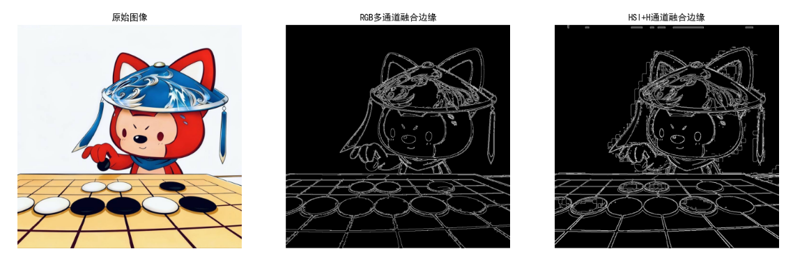

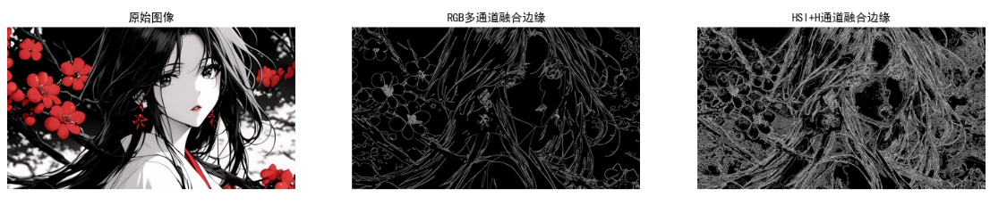
效果说明
- RGB 多通道融合:边缘更丰富(保留各颜色通道的边缘);
- HSI+H 通道融合:边缘更精准(突出颜色边界,不受亮度影响);
- 对比灰度 Canny:彩色边缘检测能捕捉更多细节(如不同颜色物体的边界)。
6.8 彩色图像中的噪声
彩色图像噪声分为「空间相关噪声」(如高斯、椒盐)和「通道相关噪声」(如色偏噪声),处理需遵循「通道同步」原则。
核心知识点
- 噪声类型:
- 高斯噪声:各通道独立分布,均值 0,标准差 σ;
- 椒盐噪声:随机出现的黑白像素,对彩色图像视觉影响更大;
- 色偏噪声:单通道噪声(如红色通道偏暗),导致图像整体偏色。
- 处理策略:
- 高斯噪声:高斯滤波、双边滤波;
- 椒盐噪声:中值滤波(首选);
- 色偏噪声:灰度世界法、直方图匹配。
代码实现:彩色图像噪声处理综合案例
import cv2
import numpy as np
import matplotlib.pyplot as plt

plt.rcParams['font.sans-serif'] = ['SimHei']
plt.rcParams['axes.unicode_minus'] = False

# 1. 添加多种噪声
def add_multi_noise(img_rgb):
    """添加高斯+椒盐+色偏噪声"""
    # 高斯噪声
    gauss_noise = np.random.normal(0, 15, img_rgb.shape)
    img_noisy = img_rgb.astype(np.float32) + gauss_noise

    # 椒盐噪声
    mask = np.random.choice([0, 1, 2], size=img_rgb.shape[:2], p=[0.01, 0.01, 0.98])
    img_noisy[mask == 0] = 0
    img_noisy[mask == 1] = 255

    # 色偏噪声(红色通道减30)
    img_noisy[:, :, 0] = np.clip(img_noisy[:, :, 0] - 30, 0, 255)

    return img_noisy.astype(np.uint8)

# 2. 噪声综合处理
def noise_removal_pipeline(img_noisy):
    """噪声处理流水线"""
    # 步骤1:中值滤波去除椒盐噪声
    img_median = cv2.medianBlur(img_noisy, 3)

    # 步骤2:双边滤波去除高斯噪声(保边)
    img_bilateral = cv2.bilateralFilter(img_median, 5, 50, 50)

    # 步骤3:灰度世界法校正色偏
    img_corrected = gray_world_balance(img_bilateral)

    return img_median, img_bilateral, img_corrected

# 3. 灰度世界法白平衡(校正色偏)
def gray_world_balance(img_rgb):
    r_mean = np.mean(img_rgb[:, :, 0])
    g_mean = np.mean(img_rgb[:, :, 1])
    b_mean = np.mean(img_rgb[:, :, 2])
    gray_mean = (r_mean + g_mean + b_mean) / 3

    # 计算增益
    r_gain = gray_mean / (r_mean + 1e-6)
    g_gain = gray_mean / (g_mean + 1e-6)
    b_gain = gray_mean / (b_mean + 1e-6)

    # 应用增益
    img_corrected = img_rgb.astype(np.float32)
    img_corrected[:, :, 0] *= r_gain
    img_corrected[:, :, 1] *= g_gain
    img_corrected[:, :, 2] *= b_gain

    return np.clip(img_corrected, 0, 255).astype(np.uint8)

# 主执行逻辑
if __name__ == "__main__":
    # 读取图像
    img_bgr = cv2.imread("test.jpg")
    img_rgb = cv2.cvtColor(img_bgr, cv2.COLOR_BGR2RGB)

    # 添加噪声
    img_noisy = add_multi_noise(img_rgb)

    # 噪声处理
    img_median, img_bilateral, img_corrected = noise_removal_pipeline(img_noisy)

    # 可视化
    plt.figure(figsize=(18, 10))
    plt.subplot(2, 2, 1)
    plt.imshow(img_rgb)
    plt.title("原始图像")
    plt.axis("off")

    plt.subplot(2, 2, 2)
    plt.imshow(img_noisy)
    plt.title("添加高斯+椒盐+色偏噪声")
    plt.axis("off")

    plt.subplot(2, 2, 3)
    plt.imshow(img_bilateral)
    plt.title("中值+双边滤波(去噪)")
    plt.axis("off")

    plt.subplot(2, 2, 4)
    plt.imshow(img_corrected)
    plt.title("灰度世界法校正色偏(最终结果)")
    plt.axis("off")
    plt.show()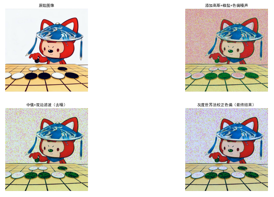
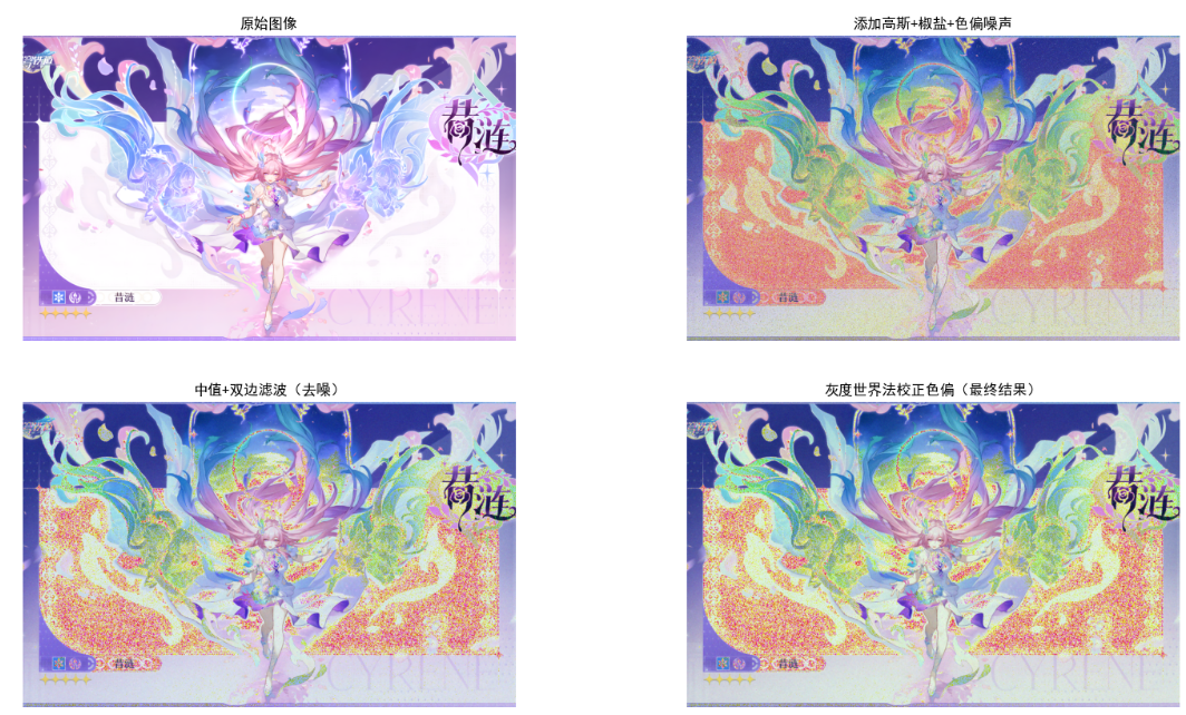
效果说明
- 中值滤波:优先去除椒盐噪声,对高斯噪声有一定抑制;
- 双边滤波:在去噪的同时保留边缘,避免图像过度模糊;
- 灰度世界法:校正色偏,使图像颜色恢复自然。
6.9 彩色图像压缩
彩色图像压缩分为「无损压缩」(如 PNG)和「有损压缩」(如 JPEG),核心思路是:
- 利用人眼对亮度敏感、对色度不敏感的特性,对色度通道下采样(如 YUV4:2:0);
- 变换编码(如 DCT)+ 熵编码(如 Huffman)降低冗余。
代码实现:彩色图像压缩(JPEG 模拟 + 下采样)
import cv2
import numpy as np
import matplotlib.pyplot as plt
import os

plt.rcParams['font.sans-serif'] = ['SimHei']
plt.rcParams['axes.unicode_minus'] = False

# 1. YUV下采样(4:4:4 → 4:2:0)
def yuv_downsampling(img_rgb):
    """
    RGB转YUV并下采样(色度通道减半)
    :param img_rgb: RGB图像
    :return: 下采样后YUV、恢复后的RGB
    """
    # RGB转YUV
    img_yuv = cv2.cvtColor(img_rgb, cv2.COLOR_RGB2YUV)

    # 分离通道
    y = img_yuv[:, :, 0]
    u = img_yuv[:, :, 1]
    v = img_yuv[:, :, 2]

    # 下采样U/V通道(4:2:0)
    u_down = cv2.resize(u, (u.shape[1]//2, u.shape[0]//2), interpolation=cv2.INTER_LINEAR)
    v_down = cv2.resize(v, (v.shape[1]//2, v.shape[0]//2), interpolation=cv2.INTER_LINEAR)

    # 恢复U/V通道尺寸
    u_up = cv2.resize(u_down, (u.shape[1], u.shape[0]), interpolation=cv2.INTER_LINEAR)
    v_up = cv2.resize(v_down, (v.shape[1], v.shape[0]), interpolation=cv2.INTER_LINEAR)

    # 合并YUV并转回RGB
    img_yuv_up = np.stack([y, u_up, v_up], axis=-1)
    img_rgb_up = cv2.cvtColor(img_yuv_up, cv2.COLOR_YUV2RGB)

    return img_rgb_up

# 2. JPEG压缩模拟(调整质量因子)
def jpeg_compression(img_rgb, quality):
    """
    模拟JPEG压缩(保存为临时文件再读取)
    :param img_rgb: RGB图像
    :param quality: 压缩质量(0-100)
    :return: 压缩后图像、压缩比
    """
    # RGB转BGR(OpenCV默认)
    img_bgr = cv2.cvtColor(img_rgb, cv2.COLOR_RGB2BGR)

    # 保存为JPEG(临时文件)
    temp_file = "temp_jpeg.jpg"
    cv2.imwrite(temp_file, img_bgr, [int(cv2.IMWRITE_JPEG_QUALITY), quality])

    # 读取压缩后图像
    img_bgr_comp = cv2.imread(temp_file)
    img_rgb_comp = cv2.cvtColor(img_bgr_comp, cv2.COLOR_BGR2RGB)

    # 计算压缩比
    orig_size = os.path.getsize(temp_file.replace(".jpg", ".png"))  # 原始PNG大小
    comp_size = os.path.getsize(temp_file)
    comp_ratio = orig_size / comp_size

    # 删除临时文件
    os.remove(temp_file)

    return img_rgb_comp, comp_ratio

# 主执行逻辑
if __name__ == "__main__":
    # 读取图像
    img_bgr = cv2.imread("test.jpg")
    img_rgb = cv2.cvtColor(img_bgr, cv2.COLOR_BGR2RGB)

    # YUV下采样压缩
    img_yuv_comp = yuv_downsampling(img_rgb)

    # JPEG压缩(质量50、20)
    img_jpeg_50, ratio_50 = jpeg_compression(img_rgb, 50)
    img_jpeg_20, ratio_20 = jpeg_compression(img_rgb, 20)

    # 可视化
    plt.figure(figsize=(18, 12))
    plt.subplot(2, 2, 1)
    plt.imshow(img_rgb)
    plt.title(f"原始图像(大小:{os.path.getsize('test.jpg')/1024:.2f}KB)")
    plt.axis("off")

    plt.subplot(2, 2, 2)
    plt.imshow(img_yuv_comp)
    plt.title("YUV4:2:0下采样(无损压缩,尺寸减半)")
    plt.axis("off")

    plt.subplot(2, 2, 3)
    plt.imshow(img_jpeg_50)
    plt.title(f"JPEG压缩(质量50,压缩比:{ratio_50:.2f})")
    plt.axis("off")

    plt.subplot(2, 2, 4)
    plt.imshow(img_jpeg_20)
    plt.title(f"JPEG压缩(质量20,压缩比:{ratio_20:.2f})")
    plt.axis("off")
    plt.show()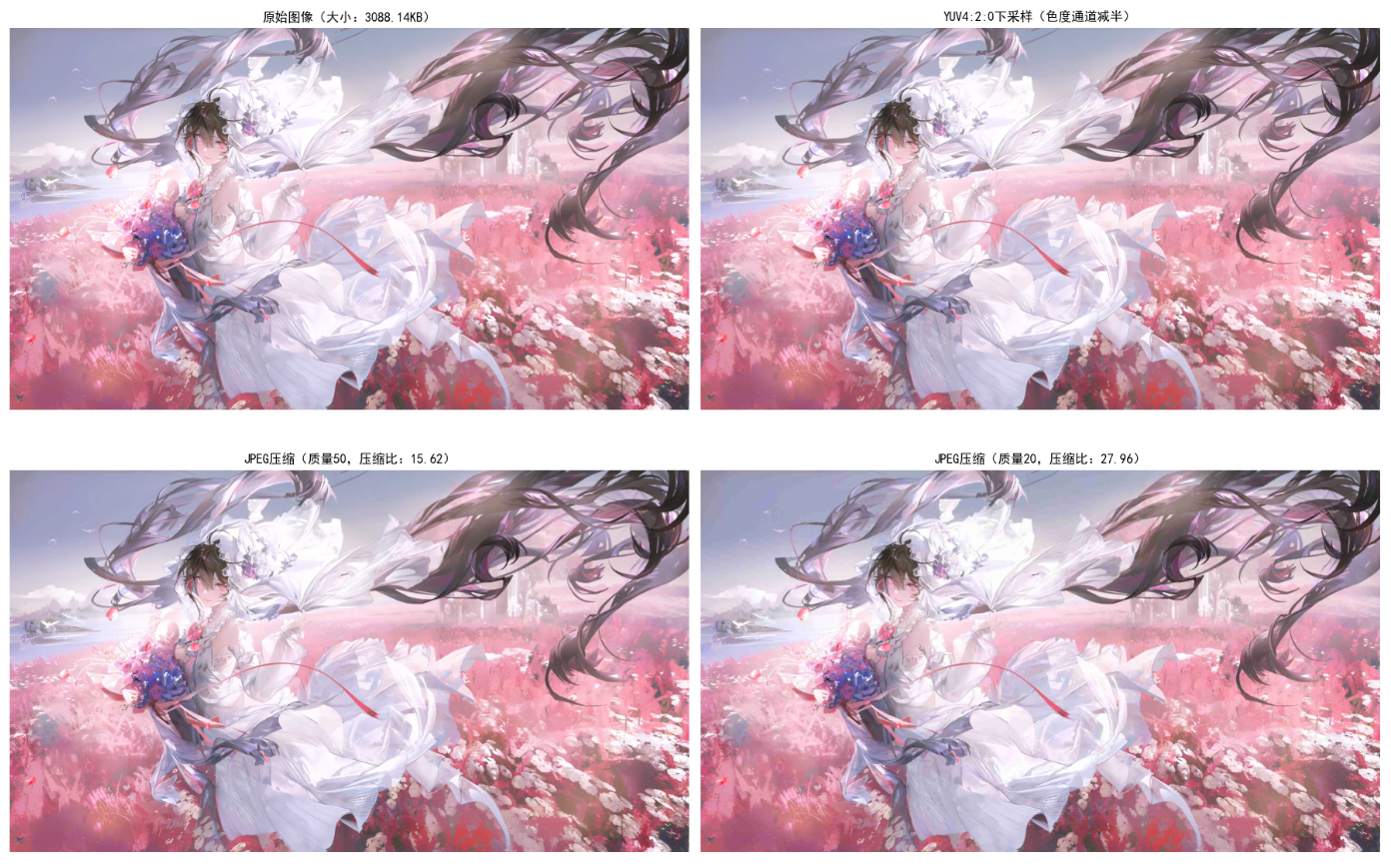
效果说明
- YUV 下采样:色度通道分辨率减半,文件大小减少约 50%,视觉质量几乎无损失;
- JPEG 压缩:质量 50 时压缩比约 5-10 倍,质量 20 时压缩比约 20-30 倍,但会出现块效应;
- 适用场景:
- 无损压缩:PNG、TIFF(适合医学影像、高精度图像);
- 有损压缩:JPEG、WebP(适合网络传输、日常照片)。
小结、参考文献和延伸读物
小结
- 彩色模型:RGB(显示)、CMY/CMYK(印刷)、HSI(处理)、CIE Lab(设备无关)是核心,需根据场景选择;
- 彩色处理原则:优先在 HSI 空间处理(分离亮度 / 色度),避免单通道操作导致颜色失真;
- 关键技术:
- 假彩色:灰度转彩色,增强视觉辨识度;
- 平滑 / 锐化:多通道同步处理,保边平滑(双边滤波)、USM 锐化是首选;
- 分割:HSI 空间分割精度高于 RGB,适合复杂场景;
- 压缩:利用人眼特性下采样色度通道,平衡压缩比和视觉质量。
参考文献
- 《数字图像处理(第四版)》------Rafael C. Gonzalez(核心教材);
- 《数字图像处理与机器视觉》------ 张铮;
- OpenCV 官方文档:https://docs.opencv.org/4.x/d6/d00/tutorial_py_root.html;
- CIE Colorimetry(国际照明委员会颜色标准)。
延伸读物
- 《颜色科学:概念与方法》------ 伯恩德・布鲁姆;
- 《JPEG 压缩原理与实现》------ 数字图像编码经典论文;
- 知乎专栏《彩色图像处理实战》------ 工业级应用案例。
习题
- 基础题:
- 实现 RGB 与 HSI 的手动转换(不调用 OpenCV),验证转换精度;
- 用 HSI 空间分割蓝色天空区域,调整 H/S/I 阈值优化分割效果。
- 进阶题:
- 实现彩色图像的自适应直方图均衡化(CLAHE),对比普通均衡化效果;
- 模拟 JPEG 压缩的 DCT 变换,分析不同质量因子对 DCT 系数的影响。
- 实战题:
- 基于彩色分割实现「红苹果计数」(统计图像中红色苹果的数量);
- 实现彩色图像的去雾算法(利用暗通道先验,处理雾天拍摄的彩色照片)。
注意事项
- 代码运行前需安装依赖:
pip install opencv-python numpy matplotlib; - 替换代码中的图像路径(如
test.jpg)为本地图像路径; - 调整阈值(如 Canny 阈值、颜色分割范围)时,需根据实际图像优化;
- 所有代码均为 Python 3.x 版本,兼容主流环境(如 Anaconda、PyCharm)。