使用pytorch进行batch_size分批训练,并使用adam+lbfgs算法
使用pytorch神经网络进行波士顿房价预测
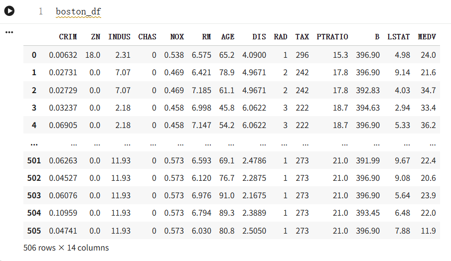
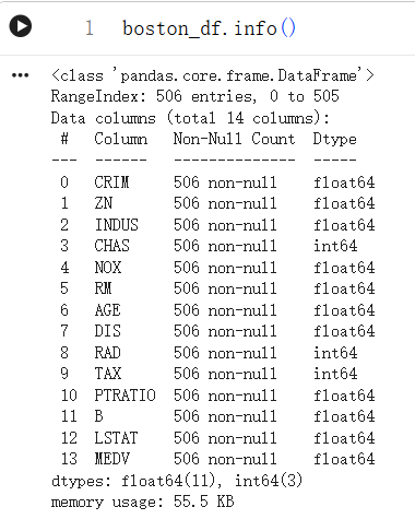
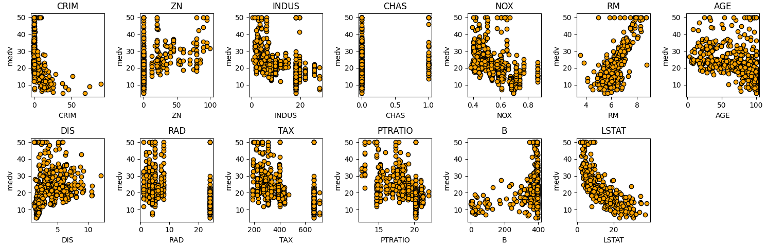
数据探索
训练过程及结果
python
import numpy as np
import pandas as pd
import matplotlib.pyplot as plt
from sklearn.model_selection import train_test_split
from sklearn.preprocessing import StandardScaler
import torch
import torch.nn as nn
import torch.optim as optim
from tqdm import tqdm
url = "https://raw.githubusercontent.com/Zhang-bingrui/Boston_house/refs/heads/main/house_data.csv"
boston_df = pd.read_csv(
url,
header=0,
on_bad_lines="skip" # 跳过格式错误的行,防止报错
)
X = boston_df.drop('MEDV', axis=1).values
y = boston_df['MEDV'].values
#划分训练集和测试集
# Veriyi %20 test setine ve %80 eğitim setine bölelim
X_train, X_test, y_train, y_test = train_test_split(X, y, test_size=0.3, random_state=42)
#输入数据标准化
scaler = StandardScaler()
X_train_scaled = scaler.fit_transform(X_train)
X_test_scaled = scaler.transform(X_test)
#将数据转换为pytorch的TENSOR
X_train = torch.tensor(X_train_scaled,dtype=torch.float32)
X_test = torch.tensor(X_test_scaled,dtype=torch.float32)
y_train = torch.tensor(y_train, dtype=torch.float32).view(-1, 1)
y_test = torch.tensor(y_test, dtype=torch.float32).view(-1, 1)
#创建数据加载器
train_dataset = TensorDataset(X_train,y_train)
test_dataset = TensorDataset(X_test,y_test)
train_loader = DataLoader(train_dataset,batch_size=64,shuffle=True)
test_loader = DataLoader(test_dataset,batch_size=64,shuffle=False)
# ANN modellerini tanımlayalım
class ANN(nn.Module):
def __init__(self, input_dim):
super(ANN, self).__init__()
self.fc1 = nn.Linear(input_dim, 64)
self.fc2 = nn.Linear(64, 32)
self.fc3 = nn.Linear(32, 1)
def forward(self, x):
x = torch.relu(self.fc1(x))
x = torch.relu(self.fc2(x))
x = self.fc3(x)
return x
num_epochs = 500
switch_epoch = int(num_epochs * 0.3)
ann_model_batch = ANN(X_train.shape[1])
criterion = nn.MSELoss()
adam_optimizer = optim.Adam(ann_model_batch.parameters(), lr=0.001)
lbfgs_optimizer = optim.LBFGS(
ann_model_batch.parameters(),
lr=0.1,
max_iter=20,
history_size=100,
line_search_fn='strong_wolfe'
)
train_losses_single = []
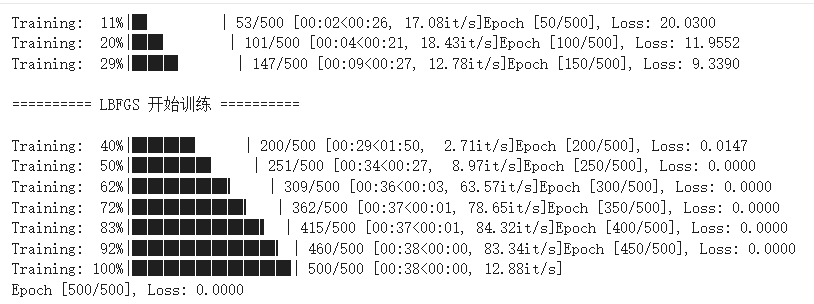
for epoch in tqdm(range(num_epochs), desc="Training"):
ann_model_batch.train()
# ===============================
# 前 30%:Adam(mini-batch)
# ===============================
if epoch < switch_epoch:
train_loss = 0.0
for inputs, targets in train_loader:
adam_optimizer.zero_grad()
outputs = ann_model_batch(inputs)
loss = criterion(outputs, targets)
loss.backward()
adam_optimizer.step()
train_loss += loss.item() * inputs.size(0)
train_loss /= len(train_loader.dataset)
# ===============================
# 后 70%:LBFGS(whole-batch)
# ===============================
else:
# 👉 只在第一次进入 LBFGS 时打印
if epoch == switch_epoch:
print("\n========== LBFGS 开始训练 ==========\n")
def closure():
lbfgs_optimizer.zero_grad()
outputs = ann_model_batch(X_train)
loss = criterion(outputs, y_train)
loss.backward()
return loss
loss = lbfgs_optimizer.step(closure)
train_loss = loss.item()
train_losses_single.append(train_loss)
if (epoch + 1) % 50 == 0:
print(f"Epoch [{epoch+1}/{num_epochs}], Loss: {train_loss:.4f}")
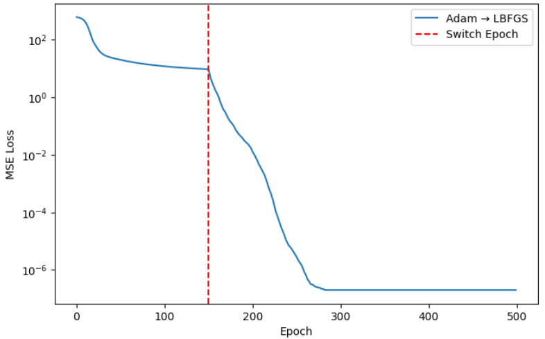
plt.figure(figsize=(8,5))
plt.plot(train_losses_single, label='Adam → LBFGS')
plt.axvline(switch_epoch, color='r', linestyle='--', label='Switch Epoch')
plt.xlabel('Epoch')
plt.ylabel('MSE Loss')
plt.yscale('log')
plt.legend()
plt.show()整批次训练与分批次训练对比
python
url = "https://raw.githubusercontent.com/Zhang-bingrui/Boston_house/refs/heads/main/house_data.csv"
boston_df = pd.read_csv(
url,
header=0,
on_bad_lines="skip" # 跳过格式错误的行,防止报错
)
# Veri setini özellikler (X) ve hedef değişken (y) olarak ayırın
X = boston_df.drop('MEDV', axis=1).values
y = boston_df['MEDV'].values
#划分训练集和测试集
# Veriyi %20 test setine ve %80 eğitim setine bölelim
X_train, X_test, y_train, y_test = train_test_split(X, y, test_size=0.2, random_state=42)
# Özellikleri ölçeklendirelim
scaler = StandardScaler()
X_train_scaled = scaler.fit_transform(X_train)
X_test_scaled = scaler.transform(X_test)
#将数据转换为pytorch的TENSOR
X_train = torch.tensor(X_train_scaled,dtype=torch.float32)
X_test = torch.tensor(X_test_scaled,dtype=torch.float32)
y_train = torch.tensor(y_train, dtype=torch.float32).view(-1, 1)
y_test = torch.tensor(y_test, dtype=torch.float32).view(-1, 1)
#创建数据加载器
train_dataset = TensorDataset(X_train,y_train)
test_dataset = TensorDataset(X_test,y_test)
train_loader = DataLoader(train_dataset,batch_size=64,shuffle=True)
test_loader = DataLoader(test_dataset,batch_size=64,shuffle=False)
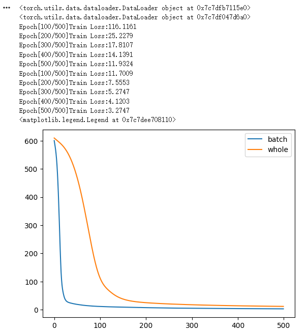
print(train_loader)
print(test_loader)
# ANN modellerini tanımlayalım
class ANN(nn.Module):
def __init__(self, input_dim):
super(ANN, self).__init__()
self.fc1 = nn.Linear(input_dim, 64)
self.fc2 = nn.Linear(64, 32)
self.fc3 = nn.Linear(32, 1)
def forward(self, x):
x = torch.relu(self.fc1(x))
x = torch.relu(self.fc2(x))
x = self.fc3(x)
return x
#整批次训练
num_epochs=500
train_losses_whole = []
#初始化模型、损失函数和优化器
ann_model_whole = ANN(X_train.shape[1])
criterion = nn.MSELoss()
optimizer = optim.Adam(ann_model_whole.parameters(), lr=0.001)
inputs = X_train
targets=y_train
for epoch in range(num_epochs):
ann_model_whole.train()
optimizer.zero_grad()
outputs = ann_model_whole(inputs)
loss = criterion(outputs, targets)
loss.backward()
optimizer.step()
train_losses_whole.append(loss.item())
if(epoch+1) % 100 == 0:
print(f'Epoch[{epoch+1}/{num_epochs}]'f'Train Loss:{loss.item():.4f}')
##-----------------------------######------------------------------------#######
# #分批次训练
train_losses_single = []
#初始化模型、损失函数和优化器
ann_model_batch = ANN(X_train.shape[1])
criterion = nn.MSELoss()
optimizer = optim.Adam(ann_model_batch.parameters(), lr=0.001)
for epoch in range(num_epochs):
#训练模式
ann_model_batch.train()
train_loss = 0.0
for inputs,targets in train_loader:
optimizer.zero_grad()
outputs = ann_model_batch(inputs)
loss = criterion(outputs,targets)
loss.backward()
optimizer.step()
train_loss += loss.item() * inputs.size(0)
#计算平均训练损失
train_loss = train_loss / len(train_loader.dataset)
train_losses_single.append(train_loss)
# #打印训练进度
if(epoch+1) % 100 == 0:
print(f'Epoch[{epoch+1}/{num_epochs}]'f'Train Loss:{train_loss:.4f}')
import matplotlib.pyplot as plt
plt.plot(train_losses_single,label='batch')
plt.plot(train_losses_whole,label='whole')
plt.legend()绘制结果对比曲线
python
# 结果验证
# ===============================
# 预测并绘制对比图
# ===============================
ann_model_batch.eval()

with torch.no_grad():
    y_train_pred = ann_model_batch(X_train).numpy().flatten()
    y_test_pred  = ann_model_batch(X_test).numpy().flatten()

y_train_true = y_train.numpy().flatten()
y_test_true  = y_test.numpy().flatten()

plt.figure(figsize=(6, 6))

# 训练集
plt.scatter(y_train_true, y_train_pred, label='Train')

# 测试集
plt.scatter(y_test_true, y_test_pred, label='Test')

# 理想预测线 y = x
min_val = min(y_train_true.min(), y_test_true.min())
max_val = max(y_train_true.max(), y_test_true.max())
plt.plot([min_val, max_val], [min_val, max_val])

plt.xlabel("True MEDV")
plt.ylabel("Predicted MEDV")
plt.title("Train vs Test Prediction Comparison")
plt.legend()
plt.grid(True)
plt.show()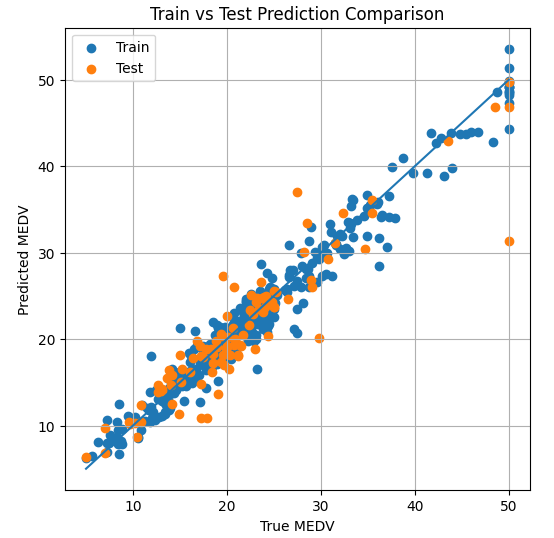
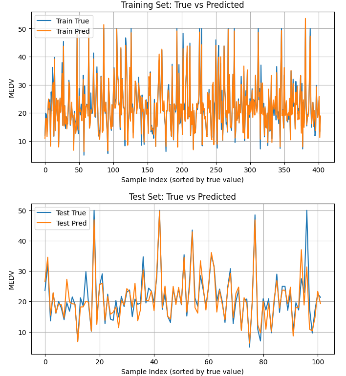
绘制无序曲线对比结果图
python
ann_model_batch.eval()

with torch.no_grad():
    y_train_pred = ann_model_batch(X_train).numpy().flatten()
    y_test_pred  = ann_model_batch(X_test).numpy().flatten()

y_train_true = y_train.numpy().flatten()
y_test_true  = y_test.numpy().flatten()
# 按真实值排序(保证曲线连续)

plt.figure(figsize=(8,4))
plt.plot(y_train_true, label='Train True')
plt.plot(y_train_pred, label='Train Pred')

plt.xlabel("Sample Index (sorted by true value)")
plt.ylabel("MEDV")
plt.title("Training Set: True vs Predicted")
plt.legend()
plt.grid(True)
plt.show()
test_idx = np.argsort(y_test_true)

plt.figure(figsize=(8,4))
plt.plot(y_test_true, label='Test True')
plt.plot(y_test_pred, label='Test Pred')

plt.xlabel("Sample Index (sorted by true value)")
plt.ylabel("MEDV")
plt.title("Test Set: True vs Predicted")
plt.legend()
plt.grid(True)
plt.show()