目录
[1. cv2.threshold()函数](#1. cv2.threshold()函数)
[2. 不同阈值类型的效果对比](#2. 不同阈值类型的效果对比)
[3. 手动选择阈值](#3. 手动选择阈值)
[4. 基于直方图的阈值选择](#4. 基于直方图的阈值选择)
[2. 自适应阈值与全局阈值的对比](#2. 自适应阈值与全局阈值的对比)
[3. 自适应阈值参数的影响](#3. 自适应阈值参数的影响)
[1. Otsu's算法的原理](#1. Otsu's算法的原理)
[2. OpenCV中的Otsu's实现](#2. OpenCV中的Otsu's实现)
[3. Otsu's算法与高斯模糊结合](#3. Otsu's算法与高斯模糊结合)
[1. 对比实验](#1. 对比实验)
[2. 优缺点对比](#2. 优缺点对比)
[1. 文档扫描](#1. 文档扫描)
[2. 硬币检测](#2. 硬币检测)
[1. 图像预处理](#1. 图像预处理)
[2. 阈值类型的选择](#2. 阈值类型的选择)
[3. 自适应阈值参数调整](#3. 自适应阈值参数调整)
[4. 多阈值分割](#4. 多阈值分割)
一、阈值分割的基本概念
阈值分割是图像处理中最基本也是最重要的技术之一,它通过将图像中像素的灰度值与一个或多个阈值进行比较,将图像分割为不同的区域(通常是前景和背景)。阈值分割广泛应用于图像预处理、目标检测、图像分割等领域。
阈值分割的基本原理
阈值分割的核心思想是:通过设定一个阈值T,将图像中的像素分为两类:
灰度值大于T的像素属于一类(通常是前景)
灰度值小于等于T的像素属于另一类(通常是背景)
数学表达式:
if f(x,y) > T: g(x,y) = 255 (白色)
else: g(x,y) = 0 (黑色)
二、全局阈值分割
全局阈值分割是指整个图像使用同一个阈值进行分割。在OpenCV中,cv2.threshold()函数用于实现全局阈值分割。
1. cv2.threshold()函数
//python
ret, dst = cv2.threshold(src, thresh, maxval, type)
参数说明:
src:输入图像(必须是灰度图像)
thresh:设定的阈值
maxval:当像素值超过阈值(或小于阈值,根据type而定)时,赋予的新值
type:阈值类型
cv2.THRESH_BINARY:二值化,大于阈值的像素设为maxval,否则设为0
cv2.THRESH_BINARY_INV:反向二值化,小于等于阈值的像素设为maxval,否则设为0
cv2.THRESH_TRUNC:截断,大于阈值的像素设为阈值,否则保持不变
cv2.THRESH_TOZERO:化零,大于阈值的像素保持不变,否则设为0
cv2.THRESH_TOZERO_INV:反向化零,小于等于阈值的像素保持不变,否则设为0
返回值:
ret:实际使用的阈值
dst:阈值分割后的图像
2. 不同阈值类型的效果对比
//python
python
import cv2

import numpy as np

from matplotlib import pyplot as plt

 #读取图像
img = cv2.imread('gradient.jpg', 0)

 #设定阈值
thresh_value = 127

maxval = 255

 #应用不同的阈值类型
ret1, thresh_binary = cv2.threshold(img, thresh_value, maxval, cv2.THRESH_BINARY)

ret2, thresh_binary_inv = cv2.threshold(img, thresh_value, maxval, cv2.THRESH_BINARY_INV)

ret3, thresh_trunc = cv2.threshold(img, thresh_value, maxval, cv2.THRESH_TRUNC)

ret4, thresh_tozero = cv2.threshold(img, thresh_value, maxval, cv2.THRESH_TOZERO)

ret5, thresh_tozero_inv = cv2.threshold(img, thresh_value, maxval, cv2.THRESH_TOZERO_INV)

 #显示结果
titles = ['Original Image', 'BINARY', 'BINARY_INV', 'TRUNC', 'TOZERO', 'TOZERO_INV']

images = [img, thresh_binary, thresh_binary_inv, thresh_trunc, thresh_tozero, thresh_tozero_inv]

plt.figure(figsize=(15, 8))

for i in range(6):

    plt.subplot(2, 3, i+1)

    plt.imshow(images[i], 'gray')

    plt.title(titles[i])

    plt.xticks([]), plt.yticks([])

plt.tight_layout()

plt.show()
3. 手动选择阈值
手动选择阈值是最基本的方法,适用于图像对比度高、直方图有明显双峰的情况。
//python
python
import cv2

import numpy as np

from matplotlib import pyplot as plt

 #读取图像

img = cv2.imread('coins.jpg', 0)

 #手动设定阈值

thresh_value = 130

maxval = 255

 #应用二值化阈值

ret, thresh = cv2.threshold(img, thresh_value, maxval, cv2.THRESH_BINARY_INV)

 #显示结果

plt.figure(figsize=(12, 6))

plt.subplot(121), plt.imshow(img, cmap='gray'), plt.title('Original Image')

plt.subplot(122), plt.imshow(thresh, cmap='gray'), plt.title(f'BINARY_INV (Thresh: {thresh_value})')

plt.tight_layout()

plt.show()
4. 基于直方图的阈值选择
通过观察图像的直方图,可以更准确地选择阈值。
//python
python
import cv2

import numpy as np

from matplotlib import pyplot as plt

 #读取图像
img = cv2.imread('coins.jpg', 0)


 #计算直方图
hist = cv2.calcHist([img], [0], None, [256], [0, 256])


 #手动设定阈值
thresh_value = 130

maxval = 255

 #应用阈值
ret, thresh = cv2.threshold(img, thresh_value, maxval, cv2.THRESH_BINARY_INV)


 #显示结果
plt.figure(figsize=(15, 6))

 #原始图像和阈值分割结果
plt.subplot(131), plt.imshow(img, cmap='gray'), plt.title('Original Image')

plt.subplot(132), plt.imshow(thresh, cmap='gray'), plt.title(f'Thresholding (T={thresh_value})')


 #直方图
plt.subplot(133)

plt.plot(hist)

plt.axvline(x=thresh_value, color='r', linestyle='')

plt.title('Image Histogram')

plt.xlabel('Pixel Value')

plt.ylabel('Frequency')

plt.xlim([0, 256])


plt.tight_layout()

plt.show()
三、自适应阈值分割
当图像的光照不均匀或存在阴影时,全局阈值分割可能会导致分割效果不佳。这时可以使用自适应阈值分割,它根据图像的局部区域动态调整阈值。
在OpenCV中,cv2.adaptiveThreshold()函数用于实现自适应阈值分割。
- cv2.adaptiveThreshold()函数
//python
dst = cv2.adaptiveThreshold(src, maxval, adaptiveMethod, thresholdType, blockSize, C)
参数说明:
src:输入图像(必须是灰度图像)
maxval:当像素值超过阈值(或小于阈值,根据thresholdType而定)时,赋予的新值
adaptiveMethod:自适应阈值计算方法
cv2.ADAPTIVE_THRESH_MEAN_C:阈值为邻域内像素的平均值减去常数C
cv2.ADAPTIVE_THRESH_GAUSSIAN_C:阈值为邻域内像素的高斯加权平均值减去常数C
thresholdType:阈值类型,只能是cv2.THRESH_BINARY或cv2.THRESH_BINARY_INV
blockSize:邻域大小(必须是奇数,如3, 5, 7...)
C:从平均值或加权平均值中减去的常数(可以是正数或负数)
2. 自适应阈值与全局阈值的对比
//python
python
import cv2

import numpy as np

from matplotlib import pyplot as plt

 #读取图像
img = cv2.imread('page.jpg', 0)

 #全局阈值
ret, thresh_global = cv2.threshold(img, 127, 255, cv2.THRESH_BINARY)

 #自适应阈值  均值法
thresh_mean = cv2.adaptiveThreshold(img, 255, cv2.ADAPTIVE_THRESH_MEAN_C,

                                   cv2.THRESH_BINARY, 11, 2)

 #自适应阈值  高斯法
thresh_gaussian = cv2.adaptiveThreshold(img, 255, cv2.ADAPTIVE_THRESH_GAUSSIAN_C,

                                       cv2.THRESH_BINARY, 11, 2)

 #显示结果
titles = ['Original Image', 'Global Thresholding (v=127)',

         'Adaptive Mean Thresholding', 'Adaptive Gaussian Thresholding']

images = [img, thresh_global, thresh_mean, thresh_gaussian]


plt.figure(figsize=(15, 10))

for i in range(4):

    plt.subplot(2, 2, i+1)

    plt.imshow(images[i], 'gray')

    plt.title(titles[i])

    plt.xticks([]), plt.yticks([])

plt.tight_layout()

plt.show()
3. 自适应阈值参数的影响
//python
python
import cv2

import numpy as np

from matplotlib import pyplot as plt

 #读取图像

img = cv2.imread('page.jpg', 0)

 #不同blockSize的效果

thresh1 = cv2.adaptiveThreshold(img, 255, cv2.ADAPTIVE_THRESH_GAUSSIAN_C,

                               cv2.THRESH_BINARY, 5, 2)

thresh2 = cv2.adaptiveThreshold(img, 255, cv2.ADAPTIVE_THRESH_GAUSSIAN_C,

                               cv2.THRESH_BINARY, 11, 2)

thresh3 = cv2.adaptiveThreshold(img, 255, cv2.ADAPTIVE_THRESH_GAUSSIAN_C,

                               cv2.THRESH_BINARY, 19, 2)


 #不同C值的效果

thresh4 = cv2.adaptiveThreshold(img, 255, cv2.ADAPTIVE_THRESH_GAUSSIAN_C,

                               cv2.THRESH_BINARY, 11, 2)

thresh5 = cv2.adaptiveThreshold(img, 255, cv2.ADAPTIVE_THRESH_GAUSSIAN_C,

                               cv2.THRESH_BINARY, 11, 2)

thresh6 = cv2.adaptiveThreshold(img, 255, cv2.ADAPTIVE_THRESH_GAUSSIAN_C,

                               cv2.THRESH_BINARY, 11, 6)


 #显示结果

plt.figure(figsize=(15, 12))

 blockSize的影响

plt.subplot(2, 3, 1), plt.imshow(thresh1, 'gray'), plt.title('blockSize=5')

plt.subplot(2, 3, 2), plt.imshow(thresh2, 'gray'), plt.title('blockSize=11')

plt.subplot(2, 3, 3), plt.imshow(thresh3, 'gray'), plt.title('blockSize=19')

 #C值的影响

plt.subplot(2, 3, 4), plt.imshow(thresh4, 'gray'), plt.title('C=2')

plt.subplot(2, 3, 5), plt.imshow(thresh5, 'gray'), plt.title('C=2')

plt.subplot(2, 3, 6), plt.imshow(thresh6, 'gray'), plt.title('C=6')

plt.tight_layout()

plt.show()
四、Otsu's自动阈值分割
Otsu's算法是一种自动阈值选择方法,它通过最大化类间方差来确定最优阈值。在OpenCV中,可以通过在cv2.threshold()函数的type参数中添加cv2.THRESH_OTSU标志来启用Otsu's算法。
1. Otsu's算法的原理
Otsu's算法的核心思想是:假设图像的直方图是双峰的,将图像分为前景和背景两部分,通过最大化这两部分的类间方差来确定最优阈值。
类间方差公式:
sigma_b^2 = w0 w1 (mu0 mu1)^2
其中:
w0:背景像素的比例
w1:前景像素的比例(w1 = 1 w0)
mu0:背景像素的平均灰度值
mu1:前景像素的平均灰度值
2. OpenCV中的Otsu's实现
//python
python
import cv2

import numpy as np

from matplotlib import pyplot as plt

 #读取图像

img = cv2.imread('coins.jpg', 0)

 #应用Otsu's阈值分割

ret_otsu, thresh_otsu = cv2.threshold(img, 0, 255, cv2.THRESH_BINARY_INV + cv2.THRESH_OTSU)

 #应用普通全局阈值分割(使用Otsu's得到的阈值)

ret_normal, thresh_normal = cv2.threshold(img, ret_otsu, 255, cv2.THRESH_BINARY_INV)

 #显示结果

plt.figure(figsize=(15, 6))

 #原始图像和直方图

plt.subplot(131), plt.imshow(img, cmap='gray'), plt.title('Original Image')

 #阈值分割结果

plt.subplot(132), plt.imshow(thresh_normal, cmap='gray'), plt.title(f'Global Thresholding (T={ret_otsu})')

plt.subplot(133), plt.imshow(thresh_otsu, cmap='gray'), plt.title(f'Otsu\'s Thresholding (T={ret_otsu})')

plt.tight_layout()

plt.show()

 显示直方图和Otsu's阈值

plt.figure(figsize=(10, 5))

hist = cv2.calcHist([img], [0], None, [256], [0, 256])

plt.plot(hist)

plt.axvline(x=ret_otsu, color='r', linestyle='', label=f'Otsu\'s Threshold: {ret_otsu}')

plt.title('Image Histogram with Otsu\'s Threshold')

plt.xlabel('Pixel Value')

plt.ylabel('Frequency')

plt.legend()

plt.xlim([0, 256])

plt.show()
3. Otsu's算法与高斯模糊结合
当图像噪声较大时,可以先进行高斯模糊处理,再应用Otsu's阈值分割:
//python
python
import cv2

import numpy as np

from matplotlib import pyplot as plt

 #读取图像

img = cv2.imread('noisy_image.jpg', 0)

 #直接应用Otsu's阈值分割

ret1, thresh1 = cv2.threshold(img, 0, 255, cv2.THRESH_BINARY_INV + cv2.THRESH_OTSU)

 #先高斯模糊,再应用Otsu's阈值分割

blurred = cv2.GaussianBlur(img, (5, 5), 0)

ret2, thresh2 = cv2.threshold(blurred, 0, 255, cv2.THRESH_BINARY_INV + cv2.THRESH_OTSU)

 #显示结果

plt.figure(figsize=(15, 8))

 #原始图像、直接Otsu、高斯模糊+Otsu

plt.subplot(221), plt.imshow(img, cmap='gray'), plt.title('Original Noisy Image')

plt.subplot(222), plt.imshow(thresh1, cmap='gray'), plt.title(f'Otsu\'s Thresholding (T={ret1})')

plt.subplot(223), plt.imshow(blurred, cmap='gray'), plt.title('Gaussian Blurred Image')

plt.subplot(224), plt.imshow(thresh2, cmap='gray'), plt.title(f'Blur + Otsu\'s (T={ret2})')

plt.tight_layout()

plt.show()
五、全局阈值与自适应阈值的对比
1. 对比实验
//python
python
import cv2
import numpy as np
from matplotlib import pyplot as plt
#读取光照不均匀的图像
img = cv2.imread('uneven_lighting.jpg', 0)
#全局阈值分割
ret1, thresh1 = cv2.threshold(img, 127, 255, cv2.THRESH_BINARY)
#Otsu's阈值分割
ret2, thresh2 = cv2.threshold(img, 0, 255, cv2.THRESH_BINARY + cv2.THRESH_OTSU)
#自适应阈值分割 均值法
thresh3 = cv2.adaptiveThreshold(img, 255, cv2.ADAPTIVE_THRESH_MEAN_C,
cv2.THRESH_BINARY, 11, 2)
#自适应阈值分割 高斯法
thresh4 = cv2.adaptiveThreshold(img, 255, cv2.ADAPTIVE_THRESH_GAUSSIAN_C,
cv2.THRESH_BINARY, 11, 2)
#显示结果
plt.figure(figsize=(15, 10))
titles = ['Original Image', 'Global Thresholding (T=127)',
"Otsu's Thresholding", 'Adaptive Mean Thresholding',
'Adaptive Gaussian Thresholding']
images = [img, thresh1, thresh2, thresh3, thresh4]
for i in range(5):
plt.subplot(2, 3, i+1)
plt.imshow(images[i], 'gray')
plt.title(titles[i])
plt.xticks([]), plt.yticks([])
plt.tight_layout()
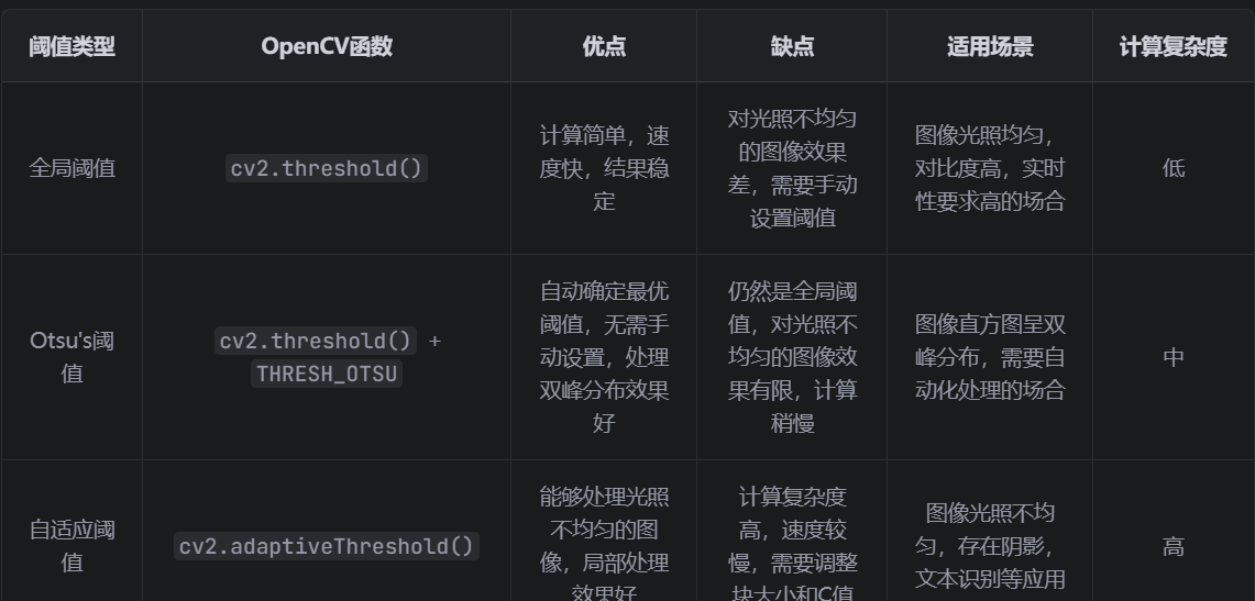
plt.show()2. 优缺点对比
六、实际应用案例
1. 文档扫描
//python
python
import cv2

import numpy as np

from matplotlib import pyplot as plt

 #读取文档图像

img = cv2.imread('document.jpg')

 #转换为灰度图像

gray = cv2.cvtColor(img, cv2.COLOR_BGR2GRAY)

 #高斯模糊,减少噪声

blurred = cv2.GaussianBlur(gray, (5, 5), 0)

 #自适应阈值分割

thresh = cv2.adaptiveThreshold(blurred, 255, cv2.ADAPTIVE_THRESH_GAUSSIAN_C,

                              cv2.THRESH_BINARY, 11, 2)

 #显示结果

plt.figure(figsize=(15, 8))

plt.subplot(131), plt.imshow(cv2.cvtColor(img, cv2.COLOR_BGR2RGB)), plt.title('Original Document')

plt.subplot(132), plt.imshow(gray, cmap='gray'), plt.title('Grayscale')

plt.subplot(133), plt.imshow(thresh, cmap='gray'), plt.title('Adaptive Thresholding')

plt.tight_layout()

plt.show()
2. 硬币检测
//python
python
import cv2

import numpy as np

from matplotlib import pyplot as plt

 #读取图像
img = cv2.imread('coins.jpg')

 #转换为灰度图像
gray = cv2.cvtColor(img, cv2.COLOR_BGR2GRAY)

 #高斯模糊
blurred = cv2.GaussianBlur(gray, (11, 11), 0)

 #Otsu's阈值分割
ret, thresh = cv2.threshold(blurred, 0, 255, cv2.THRESH_BINARY_INV + cv2.THRESH_OTSU)

 #形态学操作,去除噪声
kernel = np.ones((3, 3), np.uint8)

opening = cv2.morphologyEx(thresh, cv2.MORPH_OPEN, kernel, iterations=2)

 #检测轮廓
contours, hierarchy = cv2.findContours(opening.copy(), cv2.RETR_EXTERNAL, cv2.CHAIN_APPROX_SIMPLE)

 #绘制轮廓
img_contours = img.copy()

cv2.drawContours(img_contours, contours, 1, (0, 255, 0), 2)

 #显示结果
plt.figure(figsize=(15, 8))

plt.subplot(221), plt.imshow(cv2.cvtColor(img, cv2.COLOR_BGR2RGB)), plt.title('Original Image')

plt.subplot(222), plt.imshow(blurred, cmap='gray'), plt.title('Gaussian Blur')

plt.subplot(223), plt.imshow(thresh, cmap='gray'), plt.title(f'Otsu\'s Thresholding (T={ret})')

plt.subplot(224), plt.imshow(cv2.cvtColor(img_contours, cv2.COLOR_BGR2RGB)), plt.title(f'Coins Detected: {len(contours)}')

plt.tight_layout()

plt.show()
七、阈值分割的技巧与注意事项
1. 图像预处理
灰度转换:阈值分割只适用于灰度图像,需要先将彩色图像转换为灰度图像
噪声处理:使用高斯模糊(cv2.GaussianBlur())减少图像噪声,提高阈值分割效果
对比度增强:使用直方图均衡化(cv2.equalizeHist())增强图像对比度,使阈值分割更容易
2. 阈值类型的选择
目标为白色,背景为黑色:使用cv2.THRESH_BINARY
目标为黑色,背景为白色:使用cv2.THRESH_BINARY_INV
保留图像的亮度信息:使用cv2.THRESH_TRUNC或cv2.THRESH_TOZERO
3. 自适应阈值参数调整
blockSize:邻域大小,通常为奇数(3, 5, 7...)。值越大,阈值对局部变化越不敏感
C:从平均值或加权平均值中减去的常数。值越大,二值图像越暗;值越小,二值图像越亮
4. 多阈值分割
对于复杂图像,可以使用多阈值分割,将图像分为多个区域:
//python
python
import cv2

import numpy as np

from matplotlib import pyplot as plt

 #读取图像

img = cv2.imread('multi_threshold.jpg', 0)

 #多阈值分割

ret1, thresh1 = cv2.threshold(img, 50, 255, cv2.THRESH_BINARY)

ret2, thresh2 = cv2.threshold(img, 120, 255, cv2.THRESH_BINARY)

ret3, thresh3 = cv2.threshold(img, 180, 255, cv2.THRESH_BINARY)

 #组合多阈值结果

result = np.zeros_like(img)

result[img <= 50] = 0       #黑色

result[(img > 50) & (img <= 120)] = 85    #暗灰色

result[(img > 120) & (img <= 180)] = 170   #灰色

result[img > 180] = 255      #白色

 #显示结果

plt.figure(figsize=(15, 10))

titles = ['Original Image', 'Thresholding (T=50)',

          'Thresholding (T=120)', 'Thresholding (T=180)',

          'Multithreshold Result']

images = [img, thresh1, thresh2, thresh3, result]

for i in range(5):

    plt.subplot(2, 3, i+1)

    plt.imshow(images[i], 'gray')

    plt.title(titles[i])

    plt.xticks([]), plt.yticks([])

plt.tight_layout()

plt.show()
八、总结
阈值分割是图像处理中的基础技术,OpenCV提供了丰富的函数来实现各种阈值分割方法。
主要内容回顾
- 全局阈值分割:
使用同一个阈值处理整个图像,适用于光照均匀的图像
cv2.threshold()函数
多种阈值类型:二值化、反向二值化、截断、化零等
2. 自适应阈值分割:根据局部区域动态调整阈值,适用于光照不均匀的图像
cv2.adaptiveThreshold()函数
两种自适应方法:均值法和高斯法
3. Otsu's自动阈值:自动计算最优阈值,适用于直方图呈双峰分布的图像
在cv2.threshold()中添加cv2.THRESH_OTSU标志启用
可与高斯模糊结合使用,提高抗噪声能力
选择建议如果图像光照均匀,对比度高,选择全局阈值分割
如果图像直方图呈双峰分布,选择Otsu's阈值分割
如果图像光照不均匀或存在阴影,选择自适应阈值分割
如果图像噪声较大,先进行高斯模糊处理,再应用阈值分割
通过合理选择阈值分割方法和调整参数,可以在不同的应用场景中获得最佳的分割效果。阈值分割是许多高级图像处理任务的基础,如轮廓检测、目标识别等。