目录 💻
-
[1. 简要说明](#1. 简要说明)
-
该数据集是关于什么的?
-
本主题的重要性
-
-
[2. 关于本项目](#2. 关于本项目)
-
为什么使用CNN?
-
使用了哪些结构?
-
-
[3. 导入库](#3. 导入库)
- 本项目使用的库
-
[4. 导入数据集](#4. 导入数据集)
- 从目录调用图像
-
[5. 建模前处理](#5. 建模前处理)
-
删除不可读图像
-
绘制每个类别的随机图像
-
将数据拆分为训练集、测试集、预测集
-
为训练集、测试集、预测集创建数据框
-
计算图像比例
-
定义超参数
-
重新缩放图像
-
模型输入
-
-
[6. AlexNet](#6. AlexNet)
-
什么是AlexNet?
-
模型结构
-
输出
-
-
[7. VGGNet](#7. VGGNet)
-
什么是VGGNet?
-
模型结构
-
输出
-
-
[8. ResNet](#8. ResNet)
-
什么是ResNet?
-
模型结构
-
输出
-
-
[9. 结果](#9. 结果)
-
(准确率)与(损失)对比
-
结论
-
-
[10. 推荐主题](#10. 推荐主题)
-
如何将这些模型连接到摄像头?
-
如何为汽车构建语音报警系统?
-
简要说明
-
1. 数据集是关于什么的?
- 该数据集是关于汽车驾驶员行为检测的。这意味着什么?
驾驶员行为检测是一个研究领域,旨在识别和分析驾驶员在驾驶时的行为。在这个数据集中,我们有5个类别:1-安全驾驶,2-打电话,3-发短信,4-转弯,5-其他活动
- 该数据集是关于汽车驾驶员行为检测的。这意味着什么?
-
2. 使用了哪些结构?
- 在基于深度学习的图像分析中,有几种类型的CNN结构。在本项目中,我使用了其中三种:AlexNet、VGGNet和ResNet。这些只是图像分析任务中最常用的一些CNN结构。CNN中的每种结构都有其独特的特点和优势,正因如此,如果我们想在某个案例中使用CNN,就需要使用多种结构来比较哪一种更适合我们的图像数据。
关于本项目
-
1. 为什么使用CNN?
- CNN(卷积神经网络)是一种基于深度学习的方法,用于驾驶员行为检测。CNN是一种专门设计用于识别图像和视频中模式的神经网络。CNN在图像分类任务中特别有用,因为它们能自动学习检测图像中的边缘、角落和形状等特征。在驾驶员行为检测中,CNN用于分析驾驶员的视频片段,并识别可能表明不安全驾驶行为的模式。
-
2. 本主题的重要性
- 数据行为检测之所以重要,是因为它通过追踪用户行为和数据访问活动来帮助识别潜在的网络安全隐患。通过分析用户行为和数据访问活动,行为分析工具可以建立一个情境化的行为基线,从而区分正常与异常行为,并准确识别关键的数据威胁。
-
注意
- 本项目主要目的是展示CNN在此主题上的性能表现,并重点探讨AlexNet、VGGNet和ResNet的结构。在后续项目中,我将考虑本项目的其他部分,这些已在推荐部分(第10部分)提及。
导入库
python
import warnings
warnings.filterwarnings("ignore")
from numpy import asarray
import numpy as np
import pandas as pd
from PIL import Image
import cv2
import glob
import os
import random
import subprocess
import matplotlib.pyplot as plt
from skimage.io import imread
from matplotlib.patches import Rectangle
import tensorflow as tf
from tensorflow import keras
from tensorflow.keras import layers, models, Input, Model
from tensorflow.keras.preprocessing.image import ImageDataGenerator
from tensorflow.keras.optimizers import Adam
from tensorflow.keras.losses import BinaryCrossentropy
导入数据集
-
从目录调用图像
- 每个类别都有5个不同的文件夹。我们需要将它们分别读取到不同的变量中。为此,我创建了5个空列表,并使用 for循环 结合 os.listdir 在文件夹中进行遍历。之后,我们可以使用 if 语句来筛选并添加格式为 png 或 jpg 的图像。
您可以在下面的单元格中看到这些方法。
- 每个类别都有5个不同的文件夹。我们需要将它们分别读取到不同的变量中。为此,我创建了5个空列表,并使用 for循环 结合 os.listdir 在文件夹中进行遍历。之后,我们可以使用 if 语句来筛选并添加格式为 png 或 jpg 的图像。
python
image_list_other = []
image_list_safe = []
image_list_talking = []
image_list_text = []
image_list_turn = []

for other in os.listdir("/input/revitsone-5class/Revitsone-5classes/other_activities"):
    if other.endswith(".png") or other.endswith(".jpg"):
        image_list_other.append(os.path.join("/input/revitsone-5class/Revitsone-5classes/other_activities",
                                             other))
        print(os.path.join("/input/revitsone-5class/Revitsone-5classes/other_activities", other))

for safe in os.listdir("/input/revitsone-5class/Revitsone-5classes/safe_driving"):
    if safe.endswith(".png") or safe.endswith(".jpg"):
        image_list_safe.append(os.path.join("/input/revitsone-5class/Revitsone-5classes/safe_driving",
                                            safe))
        print(os.path.join("/input/revitsone-5class/Revitsone-5classes/safe_driving",
                           safe))

for talking in os.listdir("/input/revitsone-5class/Revitsone-5classes/talking_phone"):
    if talking.endswith(".png") or talking.endswith(".jpg"):
        image_list_talking.append(os.path.join("/input/revitsone-5class/Revitsone-5classes/talking_phone",
                                               talking))
        print(os.path.join("/input/revitsone-5class/Revitsone-5classes/talking_phone",
                           talking))

for text in os.listdir("/input/revitsone-5class/Revitsone-5classes/texting_phone"):
    if text.endswith(".png") or text.endswith(".jpg"):
        image_list_text.append(os.path.join("/input/revitsone-5class/Revitsone-5classes/texting_phone",
                                            text))
        print(os.path.join("/input/revitsone-5class/Revitsone-5classes/texting_phone",
                           text))

for turn in os.listdir("/input/revitsone-5class/Revitsone-5classes/turning"):
    if turn.endswith(".png") or turn.endswith(".jpg"):
        image_list_turn.append(os.path.join("/input/revitsone-5class/Revitsone-5classes/turning",
                                            turn))
        print(os.path.join("/input/revitsone-5class/Revitsone-5classes/turning",
                           turn))
建模前处理
-
1. 删除不可读图像
- 有时我们会遇到一些机器无法读取的不可读图像。处理这些图像有两种方法:1- 通过自己的方式查找这些图像,并在数据集中进行探索(如果数据集的图像数量较少,如本例)。2- 我们可以创建一些函数,让机器遍历图像以找出哪些图像是可读的,哪些不可读。
python
image_list_other.remove('/input/revitsone-5class/Revitsone-5classes/other_activities/img_79.jpg')
image_list_other.remove('/input/revitsone-5class/Revitsone-5classes/other_activities/img_4664.jpg')
image_list_other.remove('/input/revitsone-5class/Revitsone-5classes/other_activities/img_7973.jpg')
image_list_other.remove('/input/revitsone-5class/Revitsone-5classes/other_activities/img_13318.jpg')
image_list_other.remove('/input/revitsone-5class/Revitsone-5classes/other_activities/img_13396.jpg')
image_list_other.remove('/input/revitsone-5class/Revitsone-5classes/other_activities/img_13541.jpg')
image_list_other.remove('/input/revitsone-5class/Revitsone-5classes/other_activities/img_13625.jpg')
image_list_other.remove('/input/revitsone-5class/Revitsone-5classes/other_activities/img_20398.jpg')
image_list_other.remove('/input/revitsone-5class/Revitsone-5classes/other_activities/img_22266.jpg')

image_list_turn.remove('/input/revitsone-5class/Revitsone-5classes/turning/img_8771.jpg')
image_list_turn.remove('/input/revitsone-5class/Revitsone-5classes/turning/img_62337.jpg')
image_list_turn.remove('/input/revitsone-5class/Revitsone-5classes/turning/img_67523.jpg')
image_list_turn.remove('/input/revitsone-5class/Revitsone-5classes/turning/img_70552.jpg')
image_list_turn.remove('/input/revitsone-5class/Revitsone-5classes/turning/img_84605.jpg')
image_list_turn.remove('/input/revitsone-5class/Revitsone-5classes/turning/img_101434.jpg')
python
font = {'family':'Times New Roman','color':'#1f211f'}
background_color = '#fab72f'-
2. 绘制每个类别的随机图像
- 这部分是为了更好地理解我们拥有的图像。
python
plt.figure(1, figsize=(15, 9))
plt.axis('off')
n = 0
for i in range(4):

    n += 1
    random_img = random.choice(image_list_talking)
    imgs = imread(random_img)
    plt.suptitle("Random images of people who talk with their phone",
                 fontdict = font, fontsize=25
                 ,backgroundcolor= background_color)
    plt.subplot(2,2,n)
    plt.imshow(imgs)

plt.show()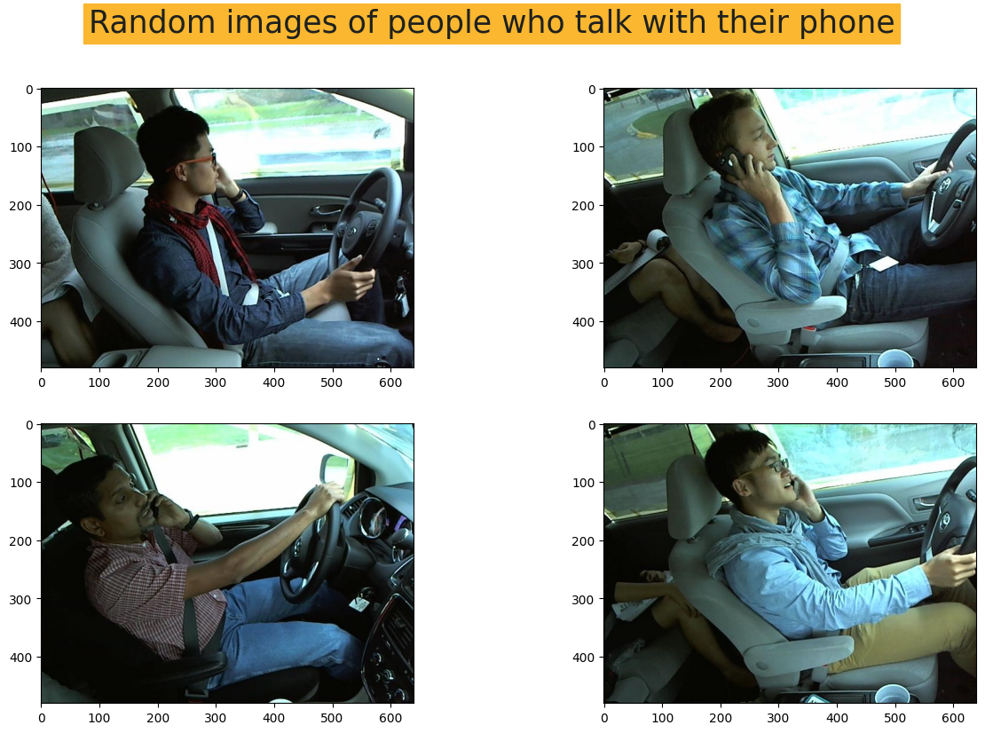
python
plt.figure(1, figsize=(15, 9))
plt.axis('off')
n = 0
for i in range(4):

    n += 1
    random_img = random.choice(image_list_text)
    imgs = imread(random_img)
    plt.suptitle("Random images of people who text with their phone",
                 fontdict = font, fontsize=25
                 ,backgroundcolor=background_color)
    plt.subplot(2,2,n)
    plt.imshow(imgs)

plt.show()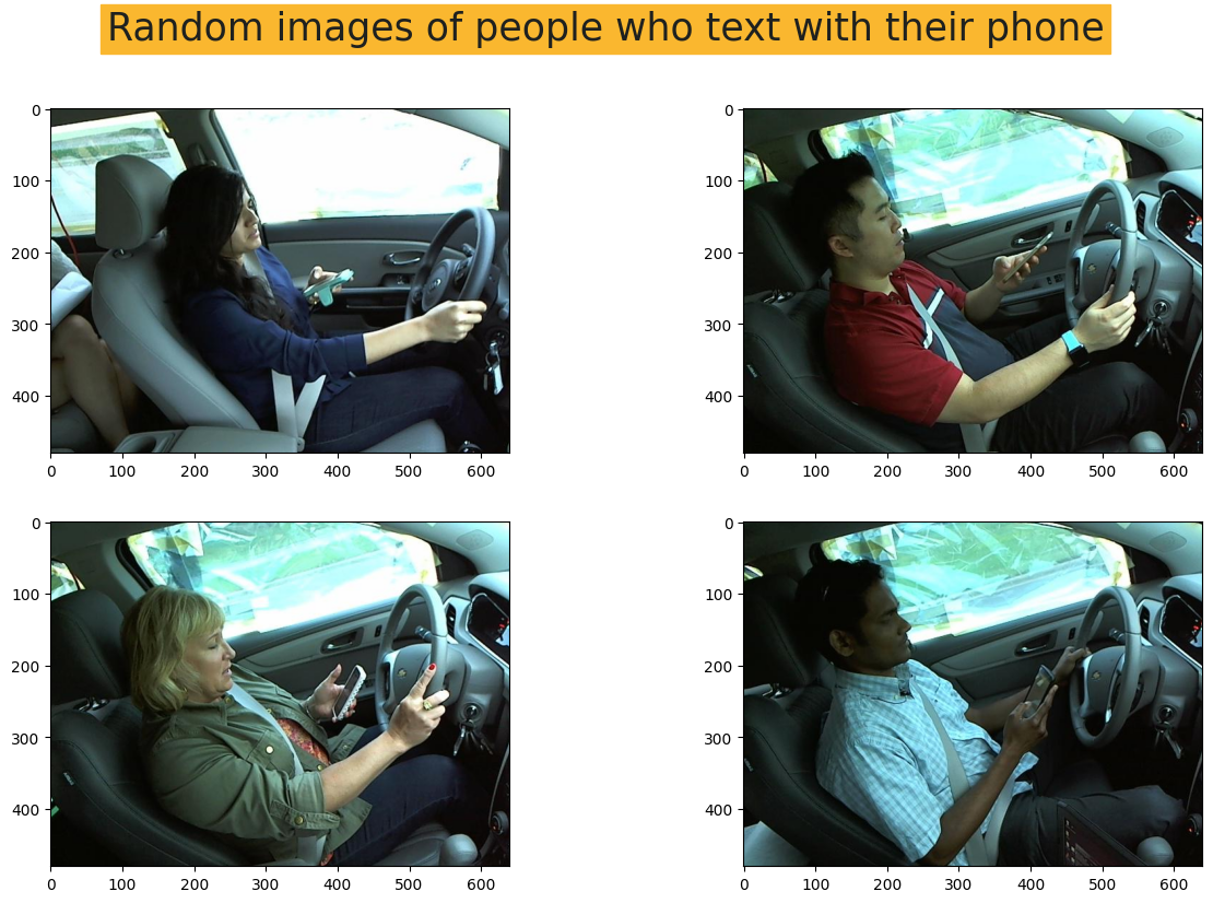
python
plt.figure(1, figsize=(15, 9))
plt.axis('off')
n = 0
for i in range(4):

    n += 1
    random_img = random.choice(image_list_turn)
    imgs = imread(random_img)
    plt.suptitle("Random images of people who turn around",
                 fontdict = font, fontsize=25
                 ,backgroundcolor=background_color)
    plt.subplot(2,2,n)
    plt.imshow(imgs)

plt.show()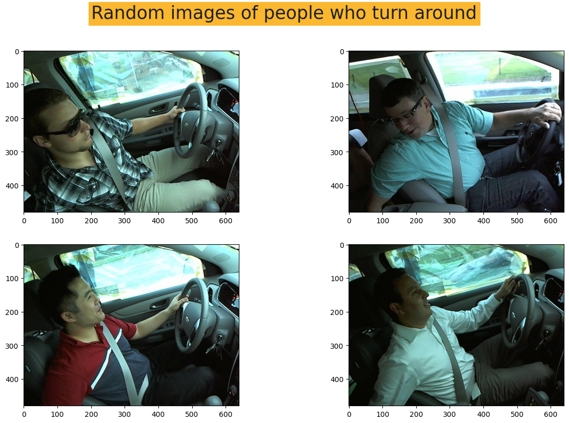
python
plt.figure(1, figsize=(15, 9))
plt.axis('off')
n = 0
for i in range(4):

    n += 1
    random_img = random.choice(image_list_safe)
    imgs = imread(random_img)
    plt.suptitle("Random images of people who drive safely",
                 fontdict = font, fontsize=25
                 ,backgroundcolor=background_color)
    plt.subplot(2,2,n)
    plt.imshow(imgs)

plt.show()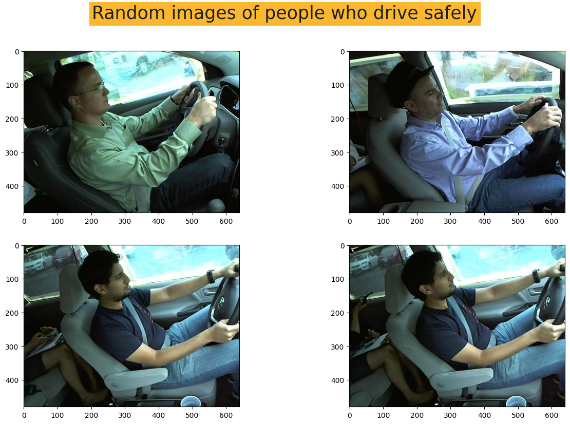
python
plt.figure(1, figsize=(15, 9))
plt.axis('off')
n = 0
for i in range(4):

    n += 1
    random_img = random.choice(image_list_other)
    imgs = imread(random_img)
    plt.suptitle("Random images of people who are in other positions",
                 fontdict = font, fontsize=25
                 ,backgroundcolor=background_color)
    plt.subplot(2,2,n)
    plt.imshow(imgs)

plt.show()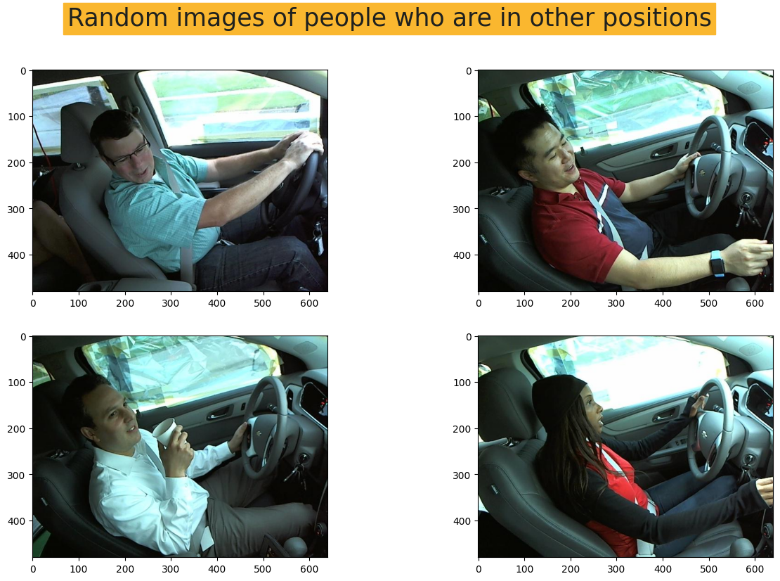
-
3. 将数据拆分为训练集、测试集、验证集
- 我决定按以下比例划分数据集:1- 训练集 = 75%,2- 测试集 = 15%,3- 验证集 = 5%
python
print("Number of samples in (Class = Other) = " ,len(image_list_other))
print("Number of samples in (Class = Safe Driving) = " ,len(image_list_safe))
print("Number of samples in (Class = Talking Phone) = " ,len(image_list_talking))
print("Number of samples in (Class = Texting Phone) = " ,len(image_list_text))
print("Number of samples in (Class = Turning) = " ,len(image_list_turn))
输出:
Number of samples in (Class = Other) =  2119
Number of samples in (Class = Safe Driving) =  2203
Number of samples in (Class = Talking Phone) =  2169
Number of samples in (Class = Texting Phone) =  2203
Number of samples in (Class = Turning) =  2057
python
print(.75*len(image_list_other) , .2*len(image_list_other) ,.05*len(image_list_other))
print(.75*len(image_list_safe) , .2*len(image_list_safe) ,.05*len(image_list_safe))
print(.75*len(image_list_talking) , .2*len(image_list_talking) ,.05*len(image_list_talking))
print(.75*len(image_list_text) , .2*len(image_list_text) ,.05*len(image_list_text))
print(.75*len(image_list_turn) , .2*len(image_list_turn) ,.05*len(image_list_turn))
输出:
1589.25 423.8 105.95
1652.25 440.6 110.15
1626.75 433.8 108.45
1652.25 440.6 110.15
1542.75 411.40000000000003 102.85000000000001
python
print("Train","Test", "Valid")

train_other = image_list_other[:1589]
test_other = image_list_other[1589:2012]
valid_other = image_list_other[2012:]

print (len(train_other), len(test_other), len(valid_other))

train_safe = image_list_safe[:1652]
test_safe = image_list_safe[1652:2092]
valid_safe = image_list_safe[2092:]

print (len(train_safe), len(test_safe), len(valid_safe))

train_talking = image_list_talking[:1626]
test_talking = image_list_talking[1626:2059]
valid_talking = image_list_talking[2059:]

print (len(train_talking), len(test_talking), len(valid_talking))

train_text = image_list_text[:1652]
test_text = image_list_text[1652:2092]
valid_text = image_list_text[2092:]

print (len(train_text), len(test_text), len(valid_text))

train_turn = image_list_turn[:1547]
test_turn = image_list_turn[1547:1959]
valid_turn = image_list_turn[1959:]

print (len(train_turn), len(test_turn), len(valid_turn))
输出:
Train Test Valid
1589 423 107
1652 440 111
1626 433 110
1652 440 111
1547 412 98-
4. 为训练集、测试集、验证集创建数据框
- 如果您不想直接从目录读取数据,而希望创建一些图像列表,您可以将数据格式转换为数据框,并使用我们将在后续单元格中看到的 flow from dataframe 方法。
为实现此方法,需要创建一个 label 列,用作标签或类别标记。
- 如果您不想直接从目录读取数据,而希望创建一些图像列表,您可以将数据格式转换为数据框,并使用我们将在后续单元格中看到的 flow from dataframe 方法。
python
train_other_df = pd.DataFrame({'image':train_other, 'label':'Other'})
train_safe_df = pd.DataFrame({'image':train_safe, 'label':'Safe'})
train_talking_df = pd.DataFrame({'image':train_talking, 'label':'Talk'})
train_text_df = pd.DataFrame({'image':train_text, 'label':'Text'})
train_turn_df = pd.DataFrame({'image':train_turn, 'label':'Turn'})
python
test_other_df = pd.DataFrame({'image':test_other, 'label':'Other'})
test_safe_df = pd.DataFrame({'image':test_safe, 'label':'Safe'})
test_talking_df = pd.DataFrame({'image':test_talking, 'label':'Talk'})
test_text_df = pd.DataFrame({'image':test_text, 'label':'Text'})
test_turn_df = pd.DataFrame({'image':test_turn, 'label':'Turn'})
python
valid_other_df = pd.DataFrame({'image':valid_other, 'label':'Other'})
valid_safe_df = pd.DataFrame({'image':valid_safe, 'label':'Safe'})
valid_talking_df = pd.DataFrame({'image':valid_talking, 'label':'Talk'})
valid_text_df = pd.DataFrame({'image':valid_text, 'label':'Text'})
valid_turn_df = pd.DataFrame({'image':valid_turn, 'label':'Turn'})
python
train_df = pd.concat([train_other_df, train_safe_df, train_talking_df, train_text_df, train_turn_df])
test_df = pd.concat([test_other_df, test_safe_df, test_talking_df, test_text_df, test_turn_df])
val_df = pd.concat([valid_other_df, valid_safe_df, valid_talking_df, valid_text_df, valid_turn_df])
python
train_df.head()
python
print("Number of rows in train dataframe is: ", len(train_df))
print("Number of rows in test dataframe is: ", len(test_df))
print("Number of rows in val dataframe is: ", len(val_df))
输出:
Number of rows in train dataframe is:  8066
Number of rows in test dataframe is:  2148
Number of rows in val dataframe is: 537-
5. 计算图像比例
- 在某些情况下,了解我们使用的图像比例非常重要。我们可以使用 cv2.imread 来完成这部分计算。
python
random_img_height = random.choice(train_other)
python
image= cv2.imread(random_img_height)

height, width= image.shape[:2]

print("The height is ", height)

print("The width is ", width)
输出:
The height is  480
The width is 640-
6. 定义超参数
- 在模型开始训练之前,需要考虑一些超参数。我将批量大小设置为64,当然您也可以使用32或其他常见数值,或者使用一些函数来检查最佳数值,但这会消耗大量运行时间,因此我只选取一些经验值。此外,对于AlexNet、ResNet和VGGNet,通常使用240*240格式作为图像高度和宽度。
python
Batch_size = 64
Img_height = 240
Img_width = 240-
7. 重新缩放图像
- 重新缩放图像并将所有图像调整为相同形状,以适应模型的输入层,这一点非常重要。
python
trainGenerator = ImageDataGenerator(rescale=1./255.)
valGenerator = ImageDataGenerator(rescale=1./255.)
testGenerator = ImageDataGenerator(rescale=1./255.)-
8. 模型输入
- 现在我们可以使用前面提到的 flow from dataframe 方法。它有助于从数据框中调用图像,并将标签指定为目标。
python
trainDataset = trainGenerator.flow_from_dataframe(
  dataframe=train_df,
  class_mode="categorical",
  x_col="image",
  y_col="label",
  batch_size=Batch_size,
  seed=42,
  shuffle=True,
  target_size=(Img_height,Img_width) #set the height and width of the images
)

testDataset = testGenerator.flow_from_dataframe(
  dataframe=test_df,
  class_mode='categorical',
  x_col="image",
  y_col="label",
  batch_size=Batch_size,
  seed=42,
  shuffle=True,
  target_size=(Img_height,Img_width)
)

valDataset = valGenerator.flow_from_dataframe(
  dataframe=val_df,
  class_mode='categorical',
  x_col="image",
  y_col="label",
  batch_size=Batch_size,
  seed=42,
  shuffle=True,
  target_size=(Img_height,Img_width)
)
输出:
Found 8066 validated image filenames belonging to 5 classes.
Found 2148 validated image filenames belonging to 5 classes.
Found 537 validated image filenames belonging to 5 classes.
AlexNet
-
1. 什么是AlexNet?
- AlexNet是一种卷积神经网络(CNN)架构,由Alex Krizhevsky、Ilya Sutskever和Geoffrey Hinton于2012年提出。它主要用于图像识别和分类任务。AlexNet是2012年ImageNet大规模视觉识别挑战赛的冠军,标志着深度学习的突破性进展。该网络包含八层;前五层是卷积层,其中一些后面跟着最大池化层,最后三层是全连接层。该网络被分成两个副本,每个在一个GPU上运行。AlexNet使用ReLU激活函数和Dropout正则化来防止过拟合。AlexNet的架构启发了自其提出以来开发的许多其他CNN架构。
-
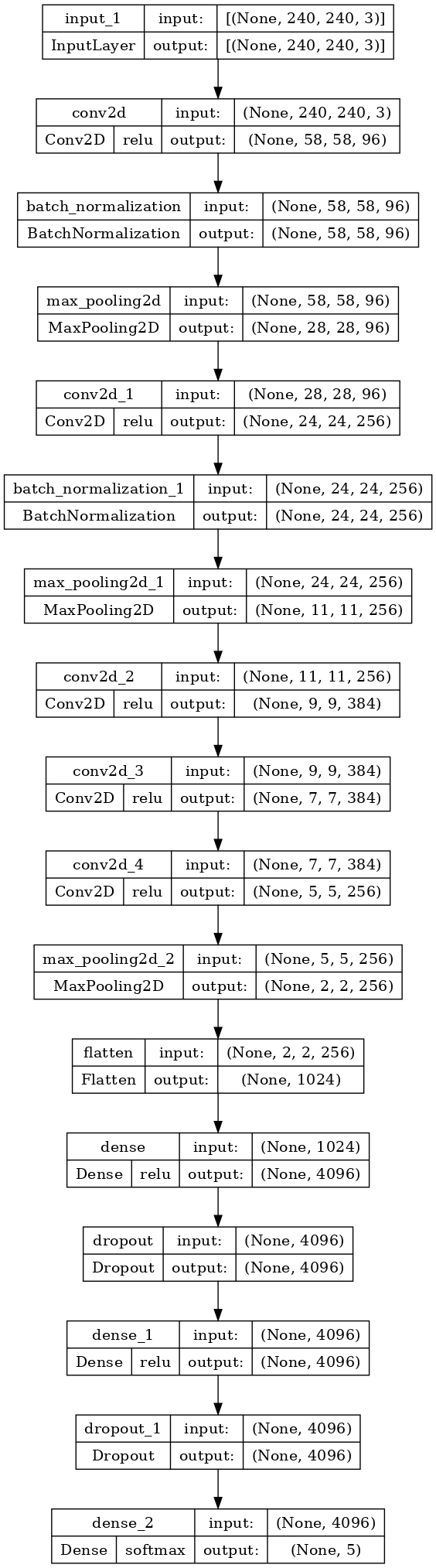
2. 模型结构
- 您可以在下面的单元格中看到AlexNet的结构。
python
def AlexNet():
    inp = layers.Input((240, 240, 3))
    x = layers.Conv2D(96, 11, 4, activation='relu')(inp)
    x = layers.BatchNormalization()(x)
    x = layers.MaxPooling2D(3, 2)(x)
    x = layers.Conv2D(256, 5, 1, activation='relu')(x)
    x = layers.BatchNormalization()(x)
    x = layers.MaxPooling2D(3, 2)(x)
    x = layers.Conv2D(384, 3, 1, activation='relu')(x)
    x = layers.Conv2D(384, 3, 1, activation='relu')(x)
    x = layers.Conv2D(256, 3, 1, activation='relu')(x)
    x = layers.MaxPooling2D(3, 2)(x)
    x = layers.Flatten()(x)
    x = layers.Dense(4096, activation='relu')(x)
    x = layers.Dropout(0.5)(x)
    x = layers.Dense(4096, activation='relu')(x)
    x = layers.Dropout(0.5)(x)
    x = layers.Dense(5, activation='softmax')(x)

    model_Alex = models.Model(inputs=inp, outputs=x)

    return model_Alex

model_Alex = AlexNet()
model_Alex.summary()
输出:
Model: "model"
_________________________________________________________________
 Layer (type)                Output Shape              Param #
=================================================================
 input_1 (InputLayer)        [(None, 240, 240, 3)]     0

 conv2d (Conv2D)             (None, 58, 58, 96)        34944

 batch_normalization (BatchN  (None, 58, 58, 96)       384
 ormalization)

 max_pooling2d (MaxPooling2D  (None, 28, 28, 96)       0
 )

 conv2d_1 (Conv2D)           (None, 24, 24, 256)       614656

 batch_normalization_1 (Batc  (None, 24, 24, 256)      1024
 hNormalization)

 max_pooling2d_1 (MaxPooling  (None, 11, 11, 256)      0
 2D)

 conv2d_2 (Conv2D)           (None, 9, 9, 384)         885120

 conv2d_3 (Conv2D)           (None, 7, 7, 384)         1327488

 conv2d_4 (Conv2D)           (None, 5, 5, 256)         884992

 max_pooling2d_2 (MaxPooling  (None, 2, 2, 256)        0
 2D)

 flatten (Flatten)           (None, 1024)              0

 dense (Dense)               (None, 4096)              4198400

 dropout (Dropout)           (None, 4096)              0

 dense_1 (Dense)             (None, 4096)              16781312

 dropout_1 (Dropout)         (None, 4096)              0

 dense_2 (Dense)             (None, 5)                 20485

=================================================================
Total params: 24,748,805
Trainable params: 24,748,101
Non-trainable params: 704
_________________________________________________________________
python
tf.keras.utils.plot_model(
    model_Alex,
    to_file='alex_model.png',
    show_shapes=True,
    show_dtype=False,
    show_layer_names=True,
    show_layer_activations=True,
    dpi=100
)
python
model_Alex.compile(loss=BinaryCrossentropy(),
              optimizer=Adam(learning_rate=0.001), metrics=['accuracy'])
python
Alex_model = model_Alex.fit(trainDataset, epochs=20, validation_data=valDataset)输出:
Epoch 1/20
127/127 [==============================] - 127s 866ms/step - loss: 0.4900 - accuracy: 0.4407 - val_loss: 0.4612 - val_accuracy: 0.4190
Epoch 2/20
127/127 [==============================] - 46s 359ms/step - loss: 0.2071 - accuracy: 0.7809 - val_loss: 0.1645 - val_accuracy: 0.8156
Epoch 3/20
127/127 [==============================] - 42s 333ms/step - loss: 0.1166 - accuracy: 0.8905 - val_loss: 0.1693 - val_accuracy: 0.8436
Epoch 4/20
127/127 [==============================] - 43s 341ms/step - loss: 0.0889 - accuracy: 0.9178 - val_loss: 0.0762 - val_accuracy: 0.9292
Epoch 5/20
127/127 [==============================] - 42s 330ms/step - loss: 0.0694 - accuracy: 0.9368 - val_loss: 0.3353 - val_accuracy: 0.7430
Epoch 6/20
127/127 [==============================] - 42s 330ms/step - loss: 0.0826 - accuracy: 0.9233 - val_loss: 0.0786 - val_accuracy: 0.9199
Epoch 7/20
127/127 [==============================] - 43s 335ms/step - loss: 0.0477 - accuracy: 0.9581 - val_loss: 0.0430 - val_accuracy: 0.9534
Epoch 8/20
127/127 [==============================] - 41s 326ms/step - loss: 0.0401 - accuracy: 0.9644 - val_loss: 0.0535 - val_accuracy: 0.9479
Epoch 9/20
127/127 [==============================] - 41s 325ms/step - loss: 0.0376 - accuracy: 0.9683 - val_loss: 0.0726 - val_accuracy: 0.9441
Epoch 10/20
127/127 [==============================] - 42s 328ms/step - loss: 0.0385 - accuracy: 0.9671 - val_loss: 0.0500 - val_accuracy: 0.9590
Epoch 11/20
127/127 [==============================] - 42s 327ms/step - loss: 0.0389 - accuracy: 0.9693 - val_loss: 0.0839 - val_accuracy: 0.9497
Epoch 12/20
127/127 [==============================] - 42s 333ms/step - loss: 0.0426 - accuracy: 0.9680 - val_loss: 0.0837 - val_accuracy: 0.9330
Epoch 13/20
127/127 [==============================] - 42s 329ms/step - loss: 0.0316 - accuracy: 0.9756 - val_loss: 0.0536 - val_accuracy: 0.9572
Epoch 14/20
127/127 [==============================] - 42s 329ms/step - loss: 0.0269 - accuracy: 0.9792 - val_loss: 0.1686 - val_accuracy: 0.9181
Epoch 15/20
127/127 [==============================] - 42s 333ms/step - loss: 0.0354 - accuracy: 0.9730 - val_loss: 0.0758 - val_accuracy: 0.9441
Epoch 16/20
127/127 [==============================] - 42s 329ms/step - loss: 0.0362 - accuracy: 0.9730 - val_loss: 0.0627 - val_accuracy: 0.9609
Epoch 17/20
127/127 [==============================] - 42s 331ms/step - loss: 0.0435 - accuracy: 0.9684 - val_loss: 0.0686 - val_accuracy: 0.9590
Epoch 18/20
127/127 [==============================] - 43s 334ms/step - loss: 0.0411 - accuracy: 0.9699 - val_loss: 0.1092 - val_accuracy: 0.9181
Epoch 19/20
127/127 [==============================] - 42s 328ms/step - loss: 0.0279 - accuracy: 0.9784 - val_loss: 0.0990 - val_accuracy: 0.9330
Epoch 20/20
127/127 [==============================] - 42s 331ms/step - loss: 0.0227 - accuracy: 0.9823 - val_loss: 0.0536 - val_accuracy: 0.9646-
3. 输出
- 我们可以绘制模型在每个训练周期的输出。为此,我们可以使用 .history 并提取 训练和验证的损失与准确率。然后我们可以绘制这两者,并了解学习的过程。
python
training_loss_alex = Alex_model.history['loss']
val_loss_alex = Alex_model.history['val_loss']
training_acc_alex = Alex_model.history['accuracy']
val_acc_alex = Alex_model.history['val_accuracy']
python
epoch_count = range(1, len(training_loss_alex) + 1)

# Visualize loss history
plt.figure(figsize=(10,5), dpi=200)
plt.plot(epoch_count, training_loss_alex, 'r--', color= 'navy')
plt.plot(epoch_count, val_loss_alex, '--bo',color= 'orangered', linewidth = '2.5', label='line with marker')
plt.legend(['Training Loss', 'Val Loss'])
plt.title('Number of epochs & Loss in ALEXNET')
plt.xlabel('Epoch')
plt.ylabel('Loss')
plt.xticks(np.arange(1,21,1))
plt.show();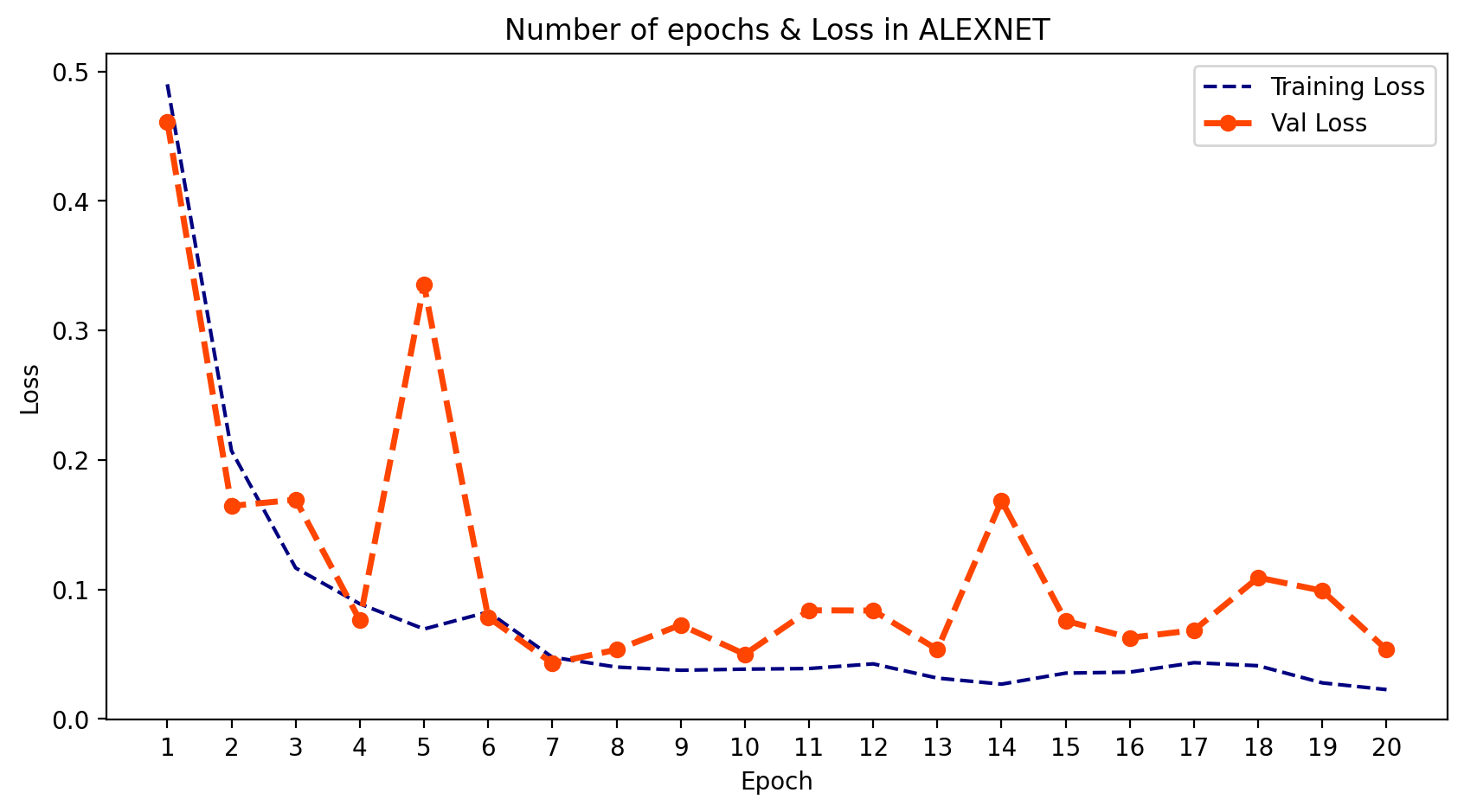
python
plt.figure(figsize=(10,5), dpi=200)
plt.plot(epoch_count, training_acc_alex, 'r--', color= 'navy')
plt.plot(epoch_count, val_acc_alex, '--bo',color= 'orangered', linewidth = '2.5', label='line with marker')
plt.legend(['Training Acc', 'Val Acc'])
plt.title('Number of epochs & Accuracy in ALEXNET')
plt.xlabel('Epoch')
plt.ylabel('Acc')
plt.xticks(np.arange(1,21,1))
plt.plot();
plt.show();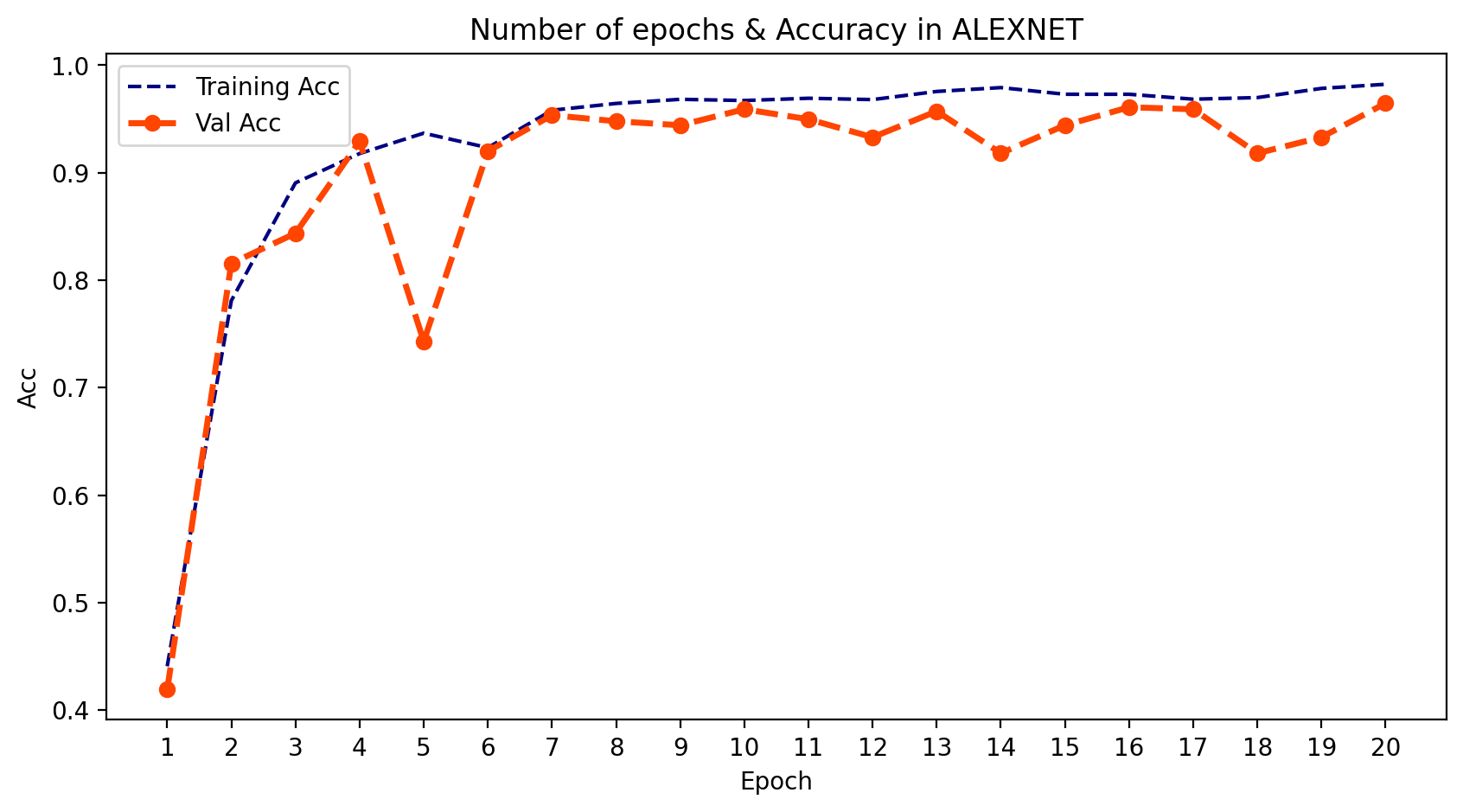
VGGNet
-
1. 什么是VGGNet?
- VGGNet,也称为视觉几何组,是一种标准的多层深度卷积神经网络(CNN)架构。"深度"指的是层数,VGG-16或VGG-19分别由16层和19层卷积层组成。VGG架构是开创性物体识别模型的基础。作为深度神经网络开发的VGGNet,在ImageNet之外的许多任务和数据集上也超越了基准模型。此外,它至今仍是最流行的图像识别架构之一。
-
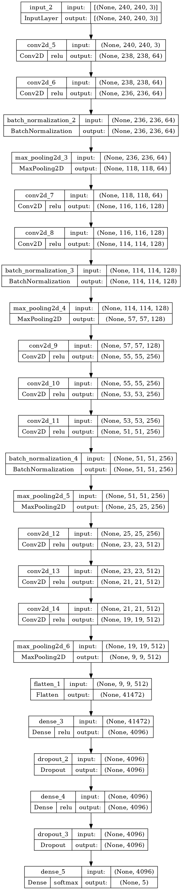
2. 模型结构
- 您可以在下面的单元格中看到VGGNet的结构。
python
def VGGNet():
    inp = layers.Input((240, 240, 3))
    x = layers.Conv2D(64, 3, 1, activation='relu')(inp)
    x = layers.Conv2D(64, 3, 1, activation='relu')(x)
    x = layers.BatchNormalization()(x)
    x = layers.MaxPooling2D(2, 2)(x)
    x = layers.Conv2D(128, 3, 1, activation='relu')(x)
    x = layers.Conv2D(128, 3, 1, activation='relu')(x)
    x = layers.BatchNormalization()(x)
    x = layers.MaxPooling2D(2, 2)(x)
    x = layers.Conv2D(256, 3, 1, activation='relu')(x)
    x = layers.Conv2D(256, 3, 1, activation='relu')(x)
    x = layers.Conv2D(256, 3, 1, activation='relu')(x)
    x = layers.BatchNormalization()(x)
    x = layers.MaxPooling2D(2, 2)(x)
    x = layers.Conv2D(512, 3, 1, activation='relu')(x)
    x = layers.Conv2D(512, 3, 1, activation='relu')(x)
    x = layers.Conv2D(512, 3, 1, activation='relu')(x)
    x = layers.MaxPooling2D(2, 2)(x)
    x = layers.Flatten()(x)
    x = layers.Dense(4096, activation='relu')(x)
    x = layers.Dropout(0.5)(x)
    x = layers.Dense(4096, activation='relu')(x)
    x = layers.Dropout(0.5)(x)
    x = layers.Dense(5, activation='softmax')(x)

    model_VGG = models.Model(inputs=inp, outputs=x)

    return model_VGG

model_VGG = VGGNet()
model_VGG.summary()
输出:
Model: "model_1"
_________________________________________________________________
 Layer (type)                Output Shape              Param #
=================================================================
 input_2 (InputLayer)        [(None, 240, 240, 3)]     0

 conv2d_5 (Conv2D)           (None, 238, 238, 64)      1792

 conv2d_6 (Conv2D)           (None, 236, 236, 64)      36928

 batch_normalization_2 (Batc  (None, 236, 236, 64)     256
 hNormalization)

 max_pooling2d_3 (MaxPooling  (None, 118, 118, 64)     0
 2D)

 conv2d_7 (Conv2D)           (None, 116, 116, 128)     73856

 conv2d_8 (Conv2D)           (None, 114, 114, 128)     147584

 batch_normalization_3 (Batc  (None, 114, 114, 128)    512
 hNormalization)

 max_pooling2d_4 (MaxPooling  (None, 57, 57, 128)      0
 2D)

 conv2d_9 (Conv2D)           (None, 55, 55, 256)       295168

 conv2d_10 (Conv2D)          (None, 53, 53, 256)       590080

 conv2d_11 (Conv2D)          (None, 51, 51, 256)       590080

 batch_normalization_4 (Batc  (None, 51, 51, 256)      1024
 hNormalization)

 max_pooling2d_5 (MaxPooling  (None, 25, 25, 256)      0
 2D)

 conv2d_12 (Conv2D)          (None, 23, 23, 512)       1180160

 conv2d_13 (Conv2D)          (None, 21, 21, 512)       2359808

 conv2d_14 (Conv2D)          (None, 19, 19, 512)       2359808

 max_pooling2d_6 (MaxPooling  (None, 9, 9, 512)        0
 2D)

 flatten_1 (Flatten)         (None, 41472)             0

 dense_3 (Dense)             (None, 4096)              169873408

 dropout_2 (Dropout)         (None, 4096)              0

 dense_4 (Dense)             (None, 4096)              16781312

 dropout_3 (Dropout)         (None, 4096)              0

 dense_5 (Dense)             (None, 5)                 20485

=================================================================
Total params: 194,312,261
Trainable params: 194,311,365
Non-trainable params: 896
_________________________________________________________________
python
tf.keras.utils.plot_model(
    model_VGG,
    to_file='vgg_model.png',
    show_shapes=True,
    show_dtype=False,
    show_layer_names=True,
    show_layer_activations=True,
    dpi=100
)
python
model_VGG.compile(loss=BinaryCrossentropy(),
              optimizer=Adam(learning_rate=0.001), metrics=['accuracy'])
python
VGG_model = model_VGG.fit(trainDataset, epochs=20, validation_data=valDataset)输出:
Epoch 1/20
127/127 [==============================] - 149s 924ms/step - loss: 1.4044 - accuracy: 0.5568 - val_loss: 0.5468 - val_accuracy: 0.3240
Epoch 2/20
127/127 [==============================] - 111s 870ms/step - loss: 0.1390 - accuracy: 0.8760 - val_loss: 0.5148 - val_accuracy: 0.3650
Epoch 3/20
127/127 [==============================] - 111s 871ms/step - loss: 0.0815 - accuracy: 0.9312 - val_loss: 0.3111 - val_accuracy: 0.6313
Epoch 4/20
127/127 [==============================] - 111s 873ms/step - loss: 0.0562 - accuracy: 0.9535 - val_loss: 0.1301 - val_accuracy: 0.8771
Epoch 5/20
127/127 [==============================] - 111s 871ms/step - loss: 0.0487 - accuracy: 0.9603 - val_loss: 0.0765 - val_accuracy: 0.9292
Epoch 6/20
127/127 [==============================] - 111s 872ms/step - loss: 0.0433 - accuracy: 0.9669 - val_loss: 0.2301 - val_accuracy: 0.8156
Epoch 7/20
127/127 [==============================] - 111s 870ms/step - loss: 0.0361 - accuracy: 0.9699 - val_loss: 0.0717 - val_accuracy: 0.9534
Epoch 8/20
127/127 [==============================] - 111s 870ms/step - loss: 0.0271 - accuracy: 0.9789 - val_loss: 0.0633 - val_accuracy: 0.9590
Epoch 9/20
127/127 [==============================] - 111s 871ms/step - loss: 0.0340 - accuracy: 0.9719 - val_loss: 0.1386 - val_accuracy: 0.8771
Epoch 10/20
127/127 [==============================] - 111s 869ms/step - loss: 0.0347 - accuracy: 0.9733 - val_loss: 0.0837 - val_accuracy: 0.9534
Epoch 11/20
127/127 [==============================] - 111s 870ms/step - loss: 0.0318 - accuracy: 0.9757 - val_loss: 0.1852 - val_accuracy: 0.8436
Epoch 12/20
127/127 [==============================] - 111s 870ms/step - loss: 0.0271 - accuracy: 0.9788 - val_loss: 0.0936 - val_accuracy: 0.9274
Epoch 13/20
127/127 [==============================] - 110s 867ms/step - loss: 0.0173 - accuracy: 0.9876 - val_loss: 0.0528 - val_accuracy: 0.9665
Epoch 14/20
127/127 [==============================] - 111s 870ms/step - loss: 0.0248 - accuracy: 0.9813 - val_loss: 0.1055 - val_accuracy: 0.9330
Epoch 15/20
127/127 [==============================] - 111s 870ms/step - loss: 0.0332 - accuracy: 0.9762 - val_loss: 0.0761 - val_accuracy: 0.9497
Epoch 16/20
127/127 [==============================] - 111s 869ms/step - loss: 0.0209 - accuracy: 0.9845 - val_loss: 0.0758 - val_accuracy: 0.9628
Epoch 17/20
127/127 [==============================] - 111s 869ms/step - loss: 0.0112 - accuracy: 0.9917 - val_loss: 0.0927 - val_accuracy: 0.9683
Epoch 18/20
127/127 [==============================] - 111s 869ms/step - loss: 0.0336 - accuracy: 0.9777 - val_loss: 0.1249 - val_accuracy: 0.9069
Epoch 19/20
127/127 [==============================] - 113s 885ms/step - loss: 0.0189 - accuracy: 0.9879 - val_loss: 0.0421 - val_accuracy: 0.9590
Epoch 20/20
127/127 [==============================] - 113s 886ms/step - loss: 0.0242 - accuracy: 0.9830 - val_loss: 0.0790 - val_accuracy: 0.9665-
3. 输出
- 我们可以绘制模型在每个训练周期的输出。为此,我们可以使用 .history 并提取 训练和验证的损失与准确率。然后我们可以绘制这两者,并了解学习的过程。
python
training_loss_vgg = VGG_model.history['loss']
val_loss_vgg = VGG_model.history['val_loss']
training_acc_vgg = VGG_model.history['accuracy']
val_acc_vgg = VGG_model.history['val_accuracy']
python
plt.figure(figsize=(10,5), dpi=200)
plt.plot(epoch_count, training_loss_vgg, 'r--', color= 'navy')
plt.plot(epoch_count, val_loss_vgg, '--bo',color= 'orangered', linewidth = '2.5', label='line with marker')
plt.legend(['Training Loss', 'Val Loss'])
plt.title('Number of epochs & Loss in VGGNET')
plt.xlabel('Epoch')
plt.ylabel('Loss')
plt.xticks(np.arange(1,21,1))
plt.show();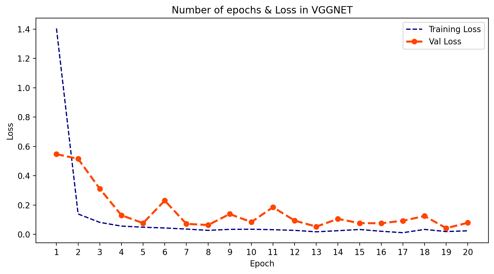
python
plt.figure(figsize=(10,5), dpi=200)
plt.plot(epoch_count, training_acc_vgg, 'r--', color= 'navy')
plt.plot(epoch_count, val_acc_vgg, '--bo',color= 'orangered', linewidth = '2.5', label='line with marker')
plt.legend(['Training Acc', 'Val Acc'])
plt.title('Number of epochs & Accuracy in VGGNET')
plt.xlabel('Epoch')
plt.ylabel('Acc')
plt.xticks(np.arange(1,21,1))
plt.plot();
plt.show();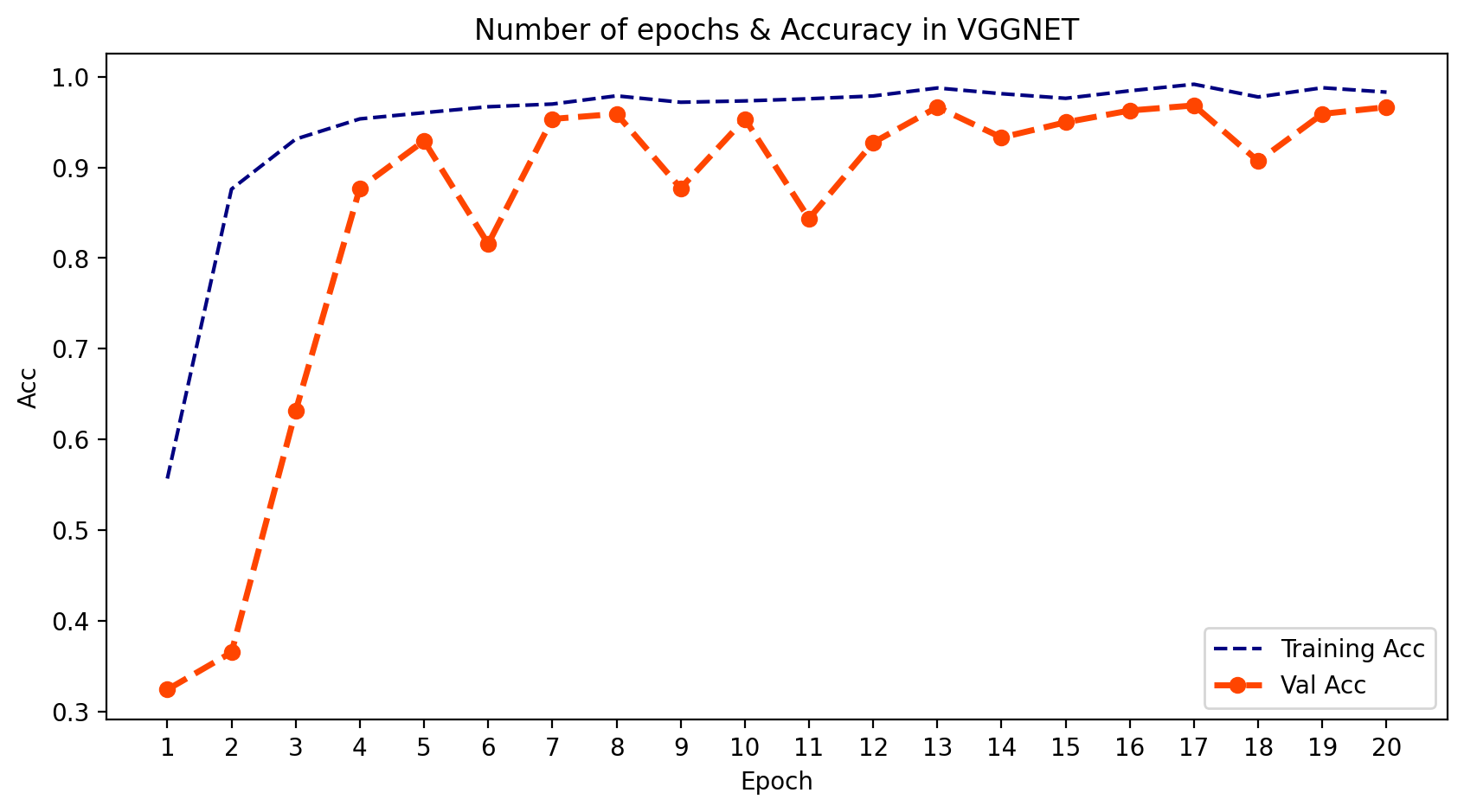
ResNet
-
1. 什么是ResNet?
- ResNet(残差网络)是一种基于深度学习的模型,它使用残差连接来提高训练性能和准确性。ResNet的架构旨在解决训练深度神经网络时出现的梯度消失问题。ResNet引入了残差块的概念,即通过跳过中间某些层,将某一层的激活连接到后续层,形成跳跃连接。这就构成了残差块,而ResNet就是通过堆叠这些残差块组成的。该网络背后的思路是,与其让网络学习基础的映射关系H(x),不如让网络去拟合残差映射F(x) := H(x) - x,从而得到H(x) := F(x) + x。跳跃连接通过跳过中间某些层,将某一层的激活与后续层相连。这使得训练非常深的神经网络时不会出现梯度消失或爆炸的问题。ResNet广泛应用于图像分类任务,并启发了自其提出以来开发的许多其他CNN架构。
-
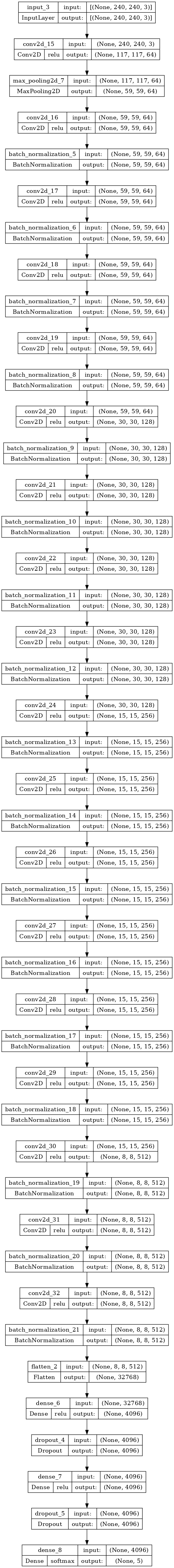
2. 模型结构
- 您可以在下面的单元格中看到ResNet的结构。
python
def ResNet34 ():
    inp = layers.Input((240, 240, 3))
    x = layers.Conv2D(64, 7, 2,padding='valid', activation='relu')(inp)
    x = layers.MaxPooling2D(strides=2, padding='same')(x)
    x = layers.Conv2D(64, 3, 1,padding='same', activation='relu')(x)
    x = layers.BatchNormalization()(x)
    x = layers.Conv2D(64, 3, 1,padding='same', activation='relu')(x)
    x = layers.BatchNormalization()(x)
    x = layers.Conv2D(64, 3, 1,padding='same', activation='relu')(x)
    x = layers.BatchNormalization()(x)
    x = layers.Conv2D(64, 3, 1,padding='same', activation='relu')(x)
    x = layers.BatchNormalization()(x)


    x = layers.Conv2D(128, 3, 2,padding='same', activation='relu')(x)
    x = layers.BatchNormalization()(x)
    x = layers.Conv2D(128, 3, 1,padding='same', activation='relu')(x)
    x = layers.BatchNormalization()(x)
    x = layers.Conv2D(128, 3, 1,padding='same', activation='relu')(x)
    x = layers.BatchNormalization()(x)
    x = layers.Conv2D(128, 3, 1,padding='same', activation='relu')(x)
    x = layers.BatchNormalization()(x)


    x = layers.Conv2D(256, 3, 2,padding='same', activation='relu')(x)
    x = layers.BatchNormalization()(x)
    x = layers.Conv2D(256, 3, 1,padding='same', activation='relu')(x)
    x = layers.BatchNormalization()(x)
    x = layers.Conv2D(256, 3, 1,padding='same', activation='relu')(x)
    x = layers.BatchNormalization()(x)
    x = layers.Conv2D(256, 3, 1,padding='same', activation='relu')(x)
    x = layers.BatchNormalization()(x)
    x = layers.Conv2D(256, 3, 1,padding='same', activation='relu')(x)
    x = layers.BatchNormalization()(x)
    x = layers.Conv2D(256, 3, 1,padding='same', activation='relu')(x)
    x = layers.BatchNormalization()(x)


    x = layers.Conv2D(512, 3, 2,padding='same', activation='relu')(x)
    x = layers.BatchNormalization()(x)
    x = layers.Conv2D(512, 3, 1,padding='same', activation='relu')(x)
    x = layers.BatchNormalization()(x)
    x = layers.Conv2D(512, 3, 1,padding='same', activation='relu')(x)
    x = layers.BatchNormalization()(x)
    x = layers.Flatten()(x)
    x = layers.Dense(4096, activation='relu')(x)
    x = layers.Dropout(0.5)(x)
    x = layers.Dense(4096, activation='relu')(x)
    x = layers.Dropout(0.5)(x)
    x = layers.Dense(5, activation='softmax')(x)


    model_Res = models.Model(inputs=inp, outputs=x)

    return model_Res

model_Res = ResNet34()
model_Res.summary()
输出:
Model: "model_2"
_________________________________________________________________
 Layer (type)                Output Shape              Param #
=================================================================
 input_3 (InputLayer)        [(None, 240, 240, 3)]     0

 conv2d_15 (Conv2D)          (None, 117, 117, 64)      9472

 max_pooling2d_7 (MaxPooling  (None, 59, 59, 64)       0
 2D)

 conv2d_16 (Conv2D)          (None, 59, 59, 64)        36928

 batch_normalization_5 (Batc  (None, 59, 59, 64)       256
 hNormalization)

 conv2d_17 (Conv2D)          (None, 59, 59, 64)        36928

 batch_normalization_6 (Batc  (None, 59, 59, 64)       256
 hNormalization)

 conv2d_18 (Conv2D)          (None, 59, 59, 64)        36928

 batch_normalization_7 (Batc  (None, 59, 59, 64)       256
 hNormalization)

 conv2d_19 (Conv2D)          (None, 59, 59, 64)        36928

 batch_normalization_8 (Batc  (None, 59, 59, 64)       256
 hNormalization)

 conv2d_20 (Conv2D)          (None, 30, 30, 128)       73856

 batch_normalization_9 (Batc  (None, 30, 30, 128)      512
 hNormalization)

 conv2d_21 (Conv2D)          (None, 30, 30, 128)       147584

 batch_normalization_10 (Bat  (None, 30, 30, 128)      512
 chNormalization)

 conv2d_22 (Conv2D)          (None, 30, 30, 128)       147584

 batch_normalization_11 (Bat  (None, 30, 30, 128)      512
 chNormalization)

 conv2d_23 (Conv2D)          (None, 30, 30, 128)       147584

 batch_normalization_12 (Bat  (None, 30, 30, 128)      512
 chNormalization)

 conv2d_24 (Conv2D)          (None, 15, 15, 256)       295168

 batch_normalization_13 (Bat  (None, 15, 15, 256)      1024
 chNormalization)

 conv2d_25 (Conv2D)          (None, 15, 15, 256)       590080

 batch_normalization_14 (Bat  (None, 15, 15, 256)      1024
 chNormalization)

 conv2d_26 (Conv2D)          (None, 15, 15, 256)       590080

 batch_normalization_15 (Bat  (None, 15, 15, 256)      1024
 chNormalization)

 conv2d_27 (Conv2D)          (None, 15, 15, 256)       590080

 batch_normalization_16 (Bat  (None, 15, 15, 256)      1024
 chNormalization)

 conv2d_28 (Conv2D)          (None, 15, 15, 256)       590080

 batch_normalization_17 (Bat  (None, 15, 15, 256)      1024
 chNormalization)

 conv2d_29 (Conv2D)          (None, 15, 15, 256)       590080

 batch_normalization_18 (Bat  (None, 15, 15, 256)      1024
 chNormalization)

 conv2d_30 (Conv2D)          (None, 8, 8, 512)         1180160

 batch_normalization_19 (Bat  (None, 8, 8, 512)        2048
 chNormalization)

 conv2d_31 (Conv2D)          (None, 8, 8, 512)         2359808

 batch_normalization_20 (Bat  (None, 8, 8, 512)        2048
 chNormalization)

 conv2d_32 (Conv2D)          (None, 8, 8, 512)         2359808

 batch_normalization_21 (Bat  (None, 8, 8, 512)        2048
 chNormalization)

 flatten_2 (Flatten)         (None, 32768)             0

 dense_6 (Dense)             (None, 4096)              134221824

 dropout_4 (Dropout)         (None, 4096)              0

 dense_7 (Dense)             (None, 4096)              16781312

 dropout_5 (Dropout)         (None, 4096)              0

 dense_8 (Dense)             (None, 5)                 20485

=================================================================
Total params: 160,858,117
Trainable params: 160,850,437
Non-trainable params: 7,680
_________________________________________________________________
python
tf.keras.utils.plot_model(
    model_Res,
    to_file='res_model.png',
    show_shapes=True,
    show_dtype=False,
    show_layer_names=True,
    show_layer_activations=True,
    dpi=100
)
python
model_Res.compile(loss=BinaryCrossentropy(),
              optimizer=Adam(learning_rate=0.001), metrics=['accuracy'])
python
RES_model = model_Res.fit(trainDataset, epochs=20, validation_data=valDataset)输出:
Epoch 1/20
127/127 [==============================] - 60s 360ms/step - loss: 0.7052 - accuracy: 0.3107 - val_loss: 0.6307 - val_accuracy: 0.2160
Epoch 2/20
127/127 [==============================] - 47s 372ms/step - loss: 0.4410 - accuracy: 0.3455 - val_loss: 0.5448 - val_accuracy: 0.2644
Epoch 3/20
127/127 [==============================] - 45s 349ms/step - loss: 0.4524 - accuracy: 0.3087 - val_loss: 0.4422 - val_accuracy: 0.3333
Epoch 4/20
127/127 [==============================] - 43s 334ms/step - loss: 0.4615 - accuracy: 0.3244 - val_loss: 0.6171 - val_accuracy: 0.3426
Epoch 5/20
127/127 [==============================] - 43s 333ms/step - loss: 0.4538 - accuracy: 0.3199 - val_loss: 0.4256 - val_accuracy: 0.3538
Epoch 6/20
127/127 [==============================] - 43s 339ms/step - loss: 0.4658 - accuracy: 0.2837 - val_loss: 0.4330 - val_accuracy: 0.3371
Epoch 7/20
127/127 [==============================] - 46s 359ms/step - loss: 0.4399 - accuracy: 0.3230 - val_loss: 0.4353 - val_accuracy: 0.3128
Epoch 8/20
127/127 [==============================] - 42s 332ms/step - loss: 0.4453 - accuracy: 0.3163 - val_loss: 0.4434 - val_accuracy: 0.3277
Epoch 9/20
127/127 [==============================] - 42s 329ms/step - loss: 0.4345 - accuracy: 0.3367 - val_loss: 0.4444 - val_accuracy: 0.3277
Epoch 10/20
127/127 [==============================] - 43s 335ms/step - loss: 0.4406 - accuracy: 0.3192 - val_loss: 0.4242 - val_accuracy: 0.3426
Epoch 11/20
127/127 [==============================] - 43s 334ms/step - loss: 0.4426 - accuracy: 0.3392 - val_loss: 0.4325 - val_accuracy: 0.3315
Epoch 12/20
127/127 [==============================] - 43s 334ms/step - loss: 0.4277 - accuracy: 0.3377 - val_loss: 0.4018 - val_accuracy: 0.3557
Epoch 13/20
127/127 [==============================] - 43s 338ms/step - loss: 0.4255 - accuracy: 0.3485 - val_loss: 0.4070 - val_accuracy: 0.3594
Epoch 14/20
127/127 [==============================] - 42s 332ms/step - loss: 0.4233 - accuracy: 0.3463 - val_loss: 0.5316 - val_accuracy: 0.3538
Epoch 15/20
127/127 [==============================] - 43s 335ms/step - loss: 0.4349 - accuracy: 0.3383 - val_loss: 0.4039 - val_accuracy: 0.3687
Epoch 16/20
127/127 [==============================] - 42s 328ms/step - loss: 0.4533 - accuracy: 0.3409 - val_loss: 0.4365 - val_accuracy: 0.3464
Epoch 17/20
127/127 [==============================] - 43s 336ms/step - loss: 0.4354 - accuracy: 0.3380 - val_loss: 3.7347 - val_accuracy: 0.2700
Epoch 18/20
127/127 [==============================] - 44s 341ms/step - loss: 0.4423 - accuracy: 0.3351 - val_loss: 0.7799 - val_accuracy: 0.3203
Epoch 19/20
127/127 [==============================] - 43s 338ms/step - loss: 0.4205 - accuracy: 0.3573 - val_loss: 0.4542 - val_accuracy: 0.3669
Epoch 20/20
127/127 [==============================] - 43s 336ms/step - loss: 0.4174 - accuracy: 0.3528 - val_loss: 0.4315 - val_accuracy: 0.3389-
3. 输出
- 我们可以绘制模型在每个训练周期的输出。为此,我们可以使用 .history 并提取 训练和验证的损失与准确率。然后我们可以绘制这两者,并了解学习的过程。
python
training_loss_res = RES_model.history['loss']
val_loss_res = RES_model.history['val_loss']
training_acc_res = RES_model.history['accuracy']
val_acc_res = RES_model.history['val_accuracy']
python
plt.figure(figsize=(10,5), dpi=200)
plt.plot(epoch_count, training_loss_res, 'r--', color= 'navy')
plt.plot(epoch_count, val_loss_res, '--bo',color= 'orangered', linewidth = '2.5', label='line with marker')
plt.legend(['Training Loss', 'Val Loss'])
plt.title('Number of epochs & Loss in RESNET34')
plt.xlabel('Epoch')
plt.ylabel('Loss')
plt.xticks(np.arange(1,21,1))
plt.show();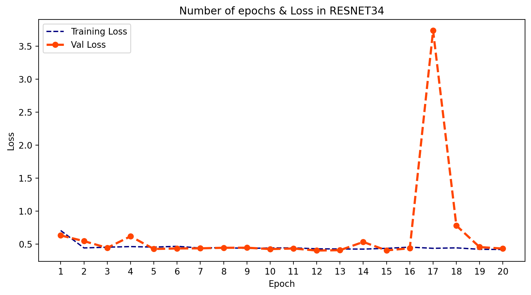
python
plt.figure(figsize=(10,5), dpi=200)
plt.plot(epoch_count, training_acc_res, 'r--', color= 'navy')
plt.plot(epoch_count, val_acc_res, '--bo',color= 'orangered', linewidth = '2.5', label='line with marker')
plt.legend(['Training Acc', 'Val Acc'])
plt.title('Number of epochs & Accuracy in RESNET34')
plt.xlabel('Epoch')
plt.ylabel('Acc')
plt.xticks(np.arange(1,21,1))
plt.plot();
plt.show();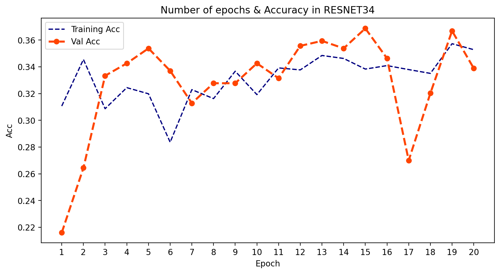
结果
-
1. (准确率)与(损失)对比
- 我们可以将所有结果放在一个图表中,比较模型输出的行为。
python
plt.figure(figsize=(10,5), dpi=200)

plt.plot(epoch_count, val_loss_alex, '--bo',color= 'navy',
         linewidth = '2.5', label='line with marker')
plt.plot(epoch_count, val_loss_vgg, '--bo',color= 'orangered',
         linewidth = '2.5', label='line with marker')
plt.plot(epoch_count, val_loss_res, '--bo',color= 'black',
         linewidth = '2.5', label='line with marker')
plt.legend(['AlexNet', 'VGGNet','ResNet'])
plt.title('Number of epochs & Loss in All Models')
plt.xlabel('Epoch')
plt.ylabel('Loss')
plt.xticks(np.arange(1,21,1))
plt.show();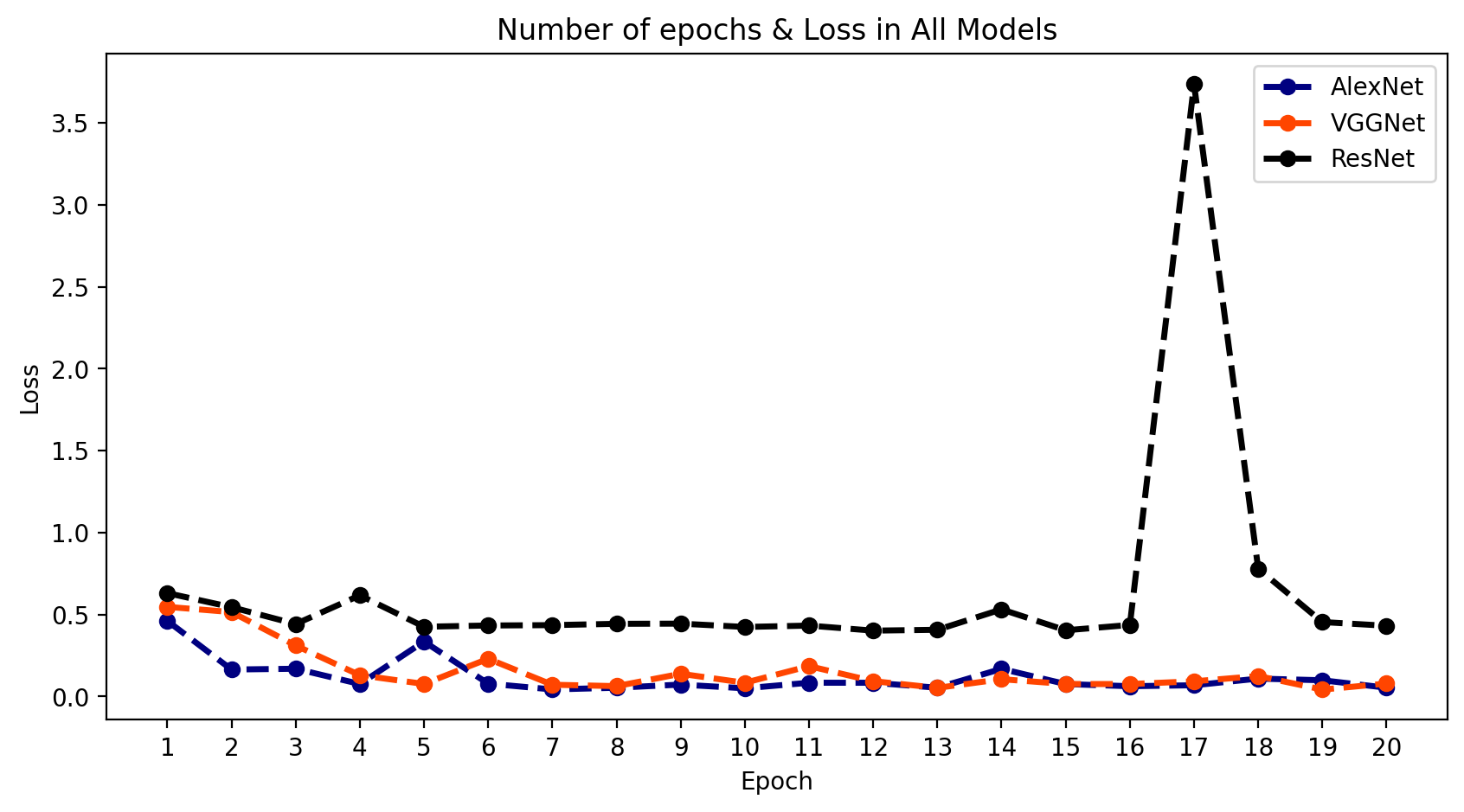
python
plt.figure(figsize=(10,5), dpi=200)

plt.plot(epoch_count, val_acc_alex, '--bo',color= 'navy',
         linewidth = '2.5', label='line with marker')
plt.plot(epoch_count, val_acc_vgg, '--bo',color= 'orangered',
         linewidth = '2.5', label='line with marker')
plt.plot(epoch_count, val_acc_res, '--bo',color= 'black',
         linewidth = '2.5', label='line with marker')
plt.legend(['AlexNet', 'VGGNet','ResNet'])
plt.title('Number of epochs & Accuracy in All Models')
plt.xlabel('Epoch')
plt.ylabel('Loss')
plt.xticks(np.arange(1,21,1))
plt.show();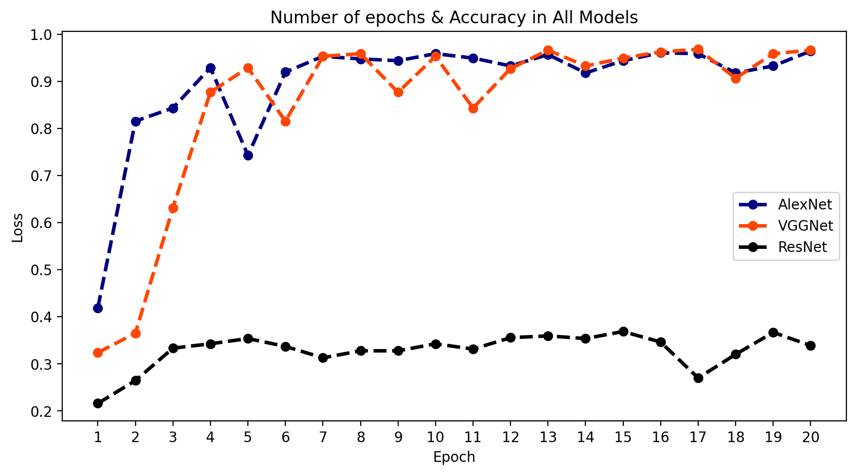
-
2. 结论
- 正如我们所看到的,AlexNet和VGGNet的结果很好,但ResNet模型拟合得不太理想。这也印证了我之前提到的为什么我们需要使用多种结构模型的原因。
推荐主题
-
1. 如何将这些模型连接到摄像头?
- 要将深度学习模型通过Python连接到摄像头,您可以使用OpenCV,这是一个开源的计算机视觉库。OpenCV提供了一个简单易用的接口,用于从摄像头捕获视频并利用深度学习模型进行实时处理。以下是入门步骤:
在您的系统上安装OpenCV和其他所需库,如TensorFlow、Keras等。
将摄像头连接到计算机,并确保其正常工作。
编写一个Python脚本,使用OpenCV从摄像头捕获视频,并利用您的深度学习模型进行处理。
运行脚本,并使用您的摄像头进行测试。
- 要将深度学习模型通过Python连接到摄像头,您可以使用OpenCV,这是一个开源的计算机视觉库。OpenCV提供了一个简单易用的接口,用于从摄像头捕获视频并利用深度学习模型进行实时处理。以下是入门步骤:
-
2. 如何为汽车构建语音报警系统?
- 要使用Python为汽车构建语音报警系统,可以按照以下步骤进行:
安装必要的库,如OpenCV、pyttsx3和threading。这些库将帮助您从摄像头捕获视频、将文本转换为语音,并同时运行多个任务。
定义一个函数,用于在检测到运动时播放语音消息。您可以使用pyttsx3创建一个引擎对象,并设置其属性,如语音、语速和音量。然后,您可以使用say方法播报消息,并使用runAndWait方法等待消息播放完成。
定义另一个函数,使用OpenCV检测运动。您可以使用cv2.VideoCapture访问摄像头,并使用cv2.cvtColor将帧转换为灰度图。接着,使用cv2.absdiff计算连续两帧之间的差异,并使用cv2.threshold将图像二值化。如果图像中的白色像素数量超过某个阈值,则表示检测到运动。
使用threading并行运行这两个函数。您可以创建两个线程对象,并将函数作为参数传递。然后,使用start方法启动线程,并使用join方法等待它们完成。
测试您的代码,并根据需要调整参数。您可以根据自己的偏好更改阈值、语音消息或摄像头索引。
- 要使用Python为汽车构建语音报警系统,可以按照以下步骤进行: