目录
一、Numpy
python
import numpy as npnp.array():创建数组
np.zeros():创建充满 0 的数组
np.ones():创建充满 1 的数组
np.empty():创建数组而不初始化其值
np.eye():用于生成单位矩阵
python
x=np.array([[1,2,3],[4,5,6]])
print("x=",x)
print("x ndim=",x.ndim)    # 维度
print("x shape=",x.shape)    # 几行几列
print("x size=",x.size)    # 几个元素
print("x dtype=",x.dtype)    # 数组类型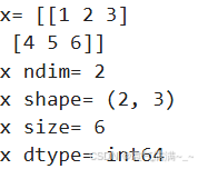
python
print("np.zeros((2,2)):\n",np.zeros((2,2)))
print("np.empty((2,3)):\n",np.empty((2,3)))
print("np.ones((2,2)):\n",np.ones((2,2)))
print("np.eye(3):\n",np.eye(3))
print("np.random.random((2,2)):\n",np.random.random((2,2)))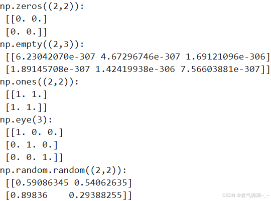
np.arange():用于生成具有固定步长的等差数列,其参数包含:
start: 起始值,默认为0。
stop: 终止值,生成的元素不包括此值。
step: 步长,默认为1。
dtype: 数据类型,默认为None,如果未提供,则使用输入数据的类型。
python
a = np.arange(12).reshape((3,4))
print(a)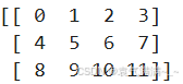
np.linspace():生成一个在指定范围内的等间隔数值序列,其参数包含:
start: 序列的起始值。
stop : 序列的结束值。如果 endpoint 为 True,该值包含在序列中;如果为 False,则不包含。
num: 要生成的样本数,默认为 50。
endpoint : 如果为 True,stop 是最后一个样本;否则,不包括 stop。默认为 True。
retstep: 如果为 True,返回 (samples, step),其中 step 是样本间隔。默认为 False。
dtype: 输出数组的类型。如果未给出,则从其他输入参数推断数据类型。
python
a = np.linspace(1,10,4) # 在[1,10]中生成等间隔数值序列
print(a)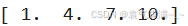
python
x=np.array([[1,2],[3,4]],dtype=np.float64)
y=np.array([[1,2],[3,4]],dtype=np.float64)
print(np.add(x,y)) # print(x+y)
print(np.subtract(x,y)) # print(x-y)
print(np.multiply(x,y)) # print(x*y)
print(np.multiply(x,x)) # print(x*x) 或 print(x**2)
# 矩阵乘法
print(x.dot(y)) # print(np.dot(x,y))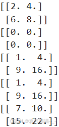
python
x=np.array([[1,2],[3,4]])
print(x)
print(x>2)
print(x==2)
print(x[x>2])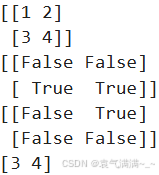
np.sum():用于计算数组元素的总和
a: 要求和的数组。
axis: 指定求和的轴。如果为None(默认值),则求整个数组的元素总和。如果为整数,则沿着指定轴求和。如果为负数,则从最后一个轴开始计数。
python
x=np.array([[1,2],[3,4]])
print(x)
print(np.sum(x))
print("sum by col:",np.sum(x,axis=0))#逐列将元素相加
print("sum by row:",np.sum(x,axis=1))#逐行将元素相加
print("min:",np.min(x))
print("每列min:",np.min(x,axis=0))
print("每行min:",np.min(x,axis=1))
print("max:",np.max(x))
print("每列max:",np.max(x,axis=0))
print("每行max:",np.max(x,axis=1))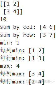
np.argmin():用于返回数组中最小值的索引
np.argmax():用于返回数组中最大值的索引
np.mean():用于返回数组的平均值
np.median():用于返回数组的中位数
np.cumsum():用于计算数组元素的累积和,这个函数可以沿着指定的轴计算累加值,如果不指定轴,则默认对数组进行展平后计算。
np.diff():用于计算数组中元素的离散差分 ,详细内容https://blog.csdn.net/weixin_42044533/article/details/115261251?fromshare=blogdetail&sharetype=blogdetail&sharerId=115261251&sharerefer=PC&sharesource=m0_74265922&sharefrom=from_link
np.nonzero():用于返回数组中非零元素的索引
np.transpose():矩阵转置
np.clip():用于将数组中的元素限制在指定的范围内
python
a = np.arange(14,2,-1).reshape(3,4)
print(a)
print("最小值索引:",np.argmin(a)) # 最小值索引
print("最大值索引:",np.argmax(a)) # 最大值索引
print("平均值:",np.mean(a)) # 平均值 print(a.mean())
print("中位数:",np.median(a)) # 中位数
print("累加和:",np.cumsum(a)) # 累加和
print(np.cumsum(a,axis=0)) # 沿着行计算累积和
print(np.cumsum(a,axis=1)) # 沿着列计算累积和
print("差分:",np.diff(a))
print(np.diff(a,axis=0))
print(np.diff(a,axis=1))
print("非零元素的索引:",np.nonzero(a))
print("排序:",np.sort(a))
print("矩阵转置:",np.transpose(a)) # 矩阵转置 print(a.T)
print(np.clip(a,5,9)) # 大于9的被置为9,小于5的被置于5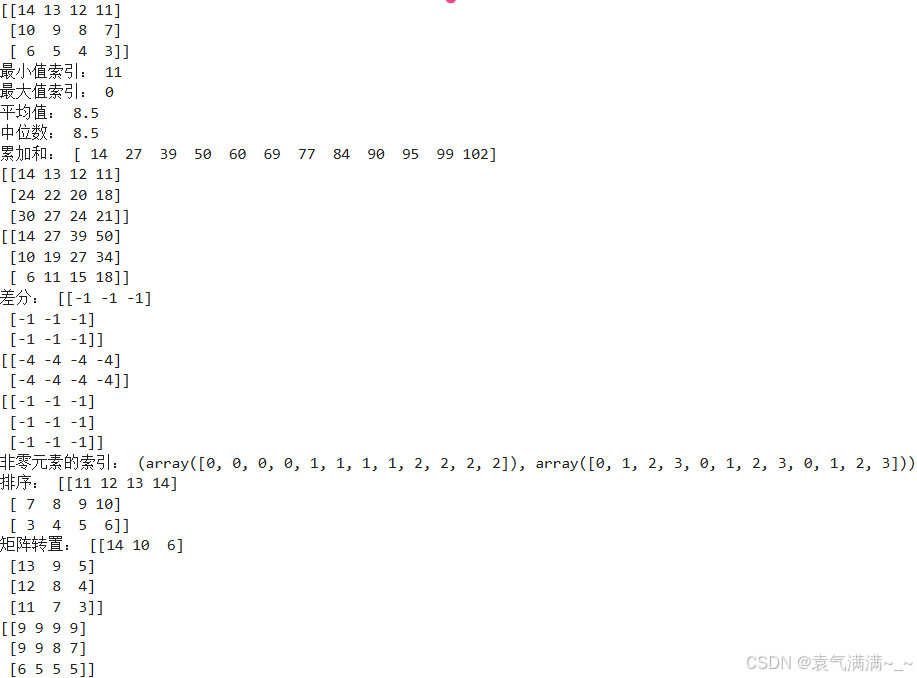
python
# 索引
x=np.array([1,2,3])
print(x[0])
x[0]=0
print(x)
np.flatten():将多维数组展平为一维数组
python
a = np.arange(3,15).reshape((3,4))
print(a)
print(a.flatten())
for col in a.flat:  # 返回了一个一维迭代器,用于访问数组中的每个元素
    print(col)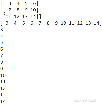
np.vstack():垂直方向上堆叠数组
np.hstack():水平方向上堆叠数组
np.concatenate():沿指定轴拼接数组
python
a = np.array([[1,2],[3,4]])
b = np.array([[1,0],[0,1]])
c = np.vstack((a,b))
d = np.hstack((a,b,a))
print(c)
print(d)

e = np.concatenate((a,b,a),axis=0)
f = np.concatenate((a,b),axis=1)
print(e)
print(f)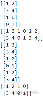
np.split():将数组沿指定轴分割为多个子数组。这个函数非常适用于需要将数据集划分为训练集和测试集,或者在机器学习任务中处理数据时。要求能够均等地分割数组。如果无法均等分割,会抛出错误。
np.array_split():将数组拆分为多个子数组。可以处理不均匀的拆分情况,即当数组长度不能被均匀分割时,最后一个子数组的长度可能会不同。
np.vsplit():沿垂直方向(行)分割成多个子数组
np.hsplit():沿水平方向(列)分割成多个子数组
python
a = np.arange(12).reshape((3,4))
print(a)
print(np.split(a,3,axis=0))
print(np.array_split(a,3,axis=1))
print(np.vsplit(a,3))
print(np.hsplit(a,2))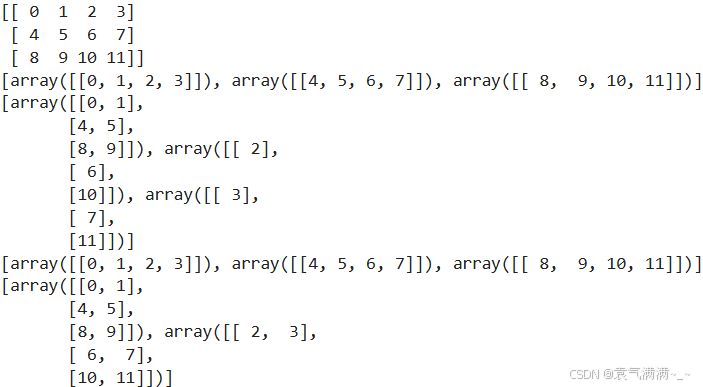
python
a = np.arange(4)
print(a)
b = a
c = b
d = a.copy() # deep copy
a[0] = 6
print("------------")
print(a)
print(b)
print(c)
print(d)
print("------------")
b[1] = 6
print(a)
print(b)
print(c)
print(d)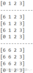
二、Pandas
python
import pandas as pdpd.Series():创建一维数组,可以存储任何数据类型(如整数、字符串、浮点数等),并且每个元素都有一个与之关联的索引(index)
python
s = pd.Series([1,3,6,np.nan,44,1])
print(s)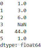
pd.DataFrame():创建一个 DataFrame 对象,支持自定义数据、索引、列名和数据类型。可以看作为一个 Excel 电子表格或者 SQL 表,或者是一个字典类型的集合。
df.describe():获取 Pandas 数据框架的描述性统计摘要,主要包含count、mean、std、min、25%、50%、75%、max这些统计信息。
df.sort_values():按某个字段中的数据进行排序
by: 指定排序的列名或列名列表。
axis: 默认值为0,表示按行排序;如果是1,将按列排序。
ascending: 布尔值或布尔值列表,指定排序的顺序,默认为升序。
inplace: 布尔值,如果为True,表示在原DataFrame上进行排序。
kind: 排序算法,默认为'quicksort',可选'mergesort'、'heapsort'和'stable'。
na_position: 处理缺失值的位置,默认为'last',表示缺失值排在最后,设置为'first'时,缺失值排在最前面。
python
dates = pd.date_range('20260101',periods=3)
print(dates)
df = pd.DataFrame(np.arange(12).reshape((3,4)),index=dates,columns=['a','b','c','d'])
print(df)
print("dtypes:\n",df.dtypes)
print("columns:",df.columns)
print("values:\n",df.values)
print("describe:\n",df.describe())
print("sort_index:\n",df.sort_index(axis=1,ascending=False))
print("sort_values:\n",df.sort_values(by='b'))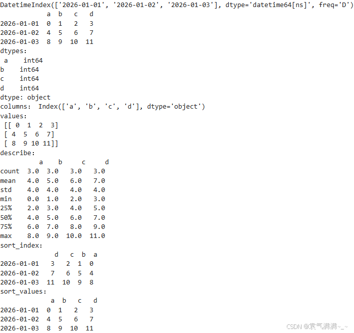
loc:基于标签的索引方式,DataFrame.loc行选择, 列选择。
iloc:通过行和列的索引位置来访问数据。
python
print(df['a']) # print(df.a)
print(df[0:2]) # print(df['2026-01-01':'2026-01-02'])
print(df.loc['2026-01-01'])
print(df.loc[:,['a','b']])
print(df.iloc[[0,2],1:3])
print(df[df.a>3])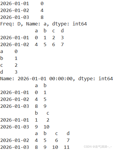
python
df.iloc[2,2] = 66
df.loc['20260101','d'] = 666
print(df)
df.b[df.a<4] = 111
print(df)
df[df.a<5] = 0
print(df)
df['e'] = 12
print(df)
df['f'] = pd.Series([13,23,33],index=pd.date_range('20260101',periods=3))
print(df)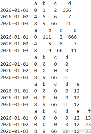
dropna():删除包含缺失值的行或列
fillna():填充 DataFrame 或 Series 中的缺失值(NaN)
isnull():检测数据中的缺失值
np.any():判断数组中是否存在至少一个元素为 True(或非零)
python
dates = pd.date_range('20260101',periods=3)
df = pd.DataFrame(np.arange(12).reshape((3,4)),index=dates,columns=['a','b','c','d'])
df.iloc[0,1] = np.nan
df.iloc[1,2] = np.nan
print(df)
print(df.dropna(axis=0,how='any'))  # how={'any','all'},为any时这一行或列有一个缺失值就要删去,为all时必须这一行或列都是缺失值才能删去
print(df.dropna(axis=0,how='all'))
print(df.dropna(axis=1,how='any'))
print(df.fillna(value=0))
print(df.isnull())
print(np.any(df.isnull())==True)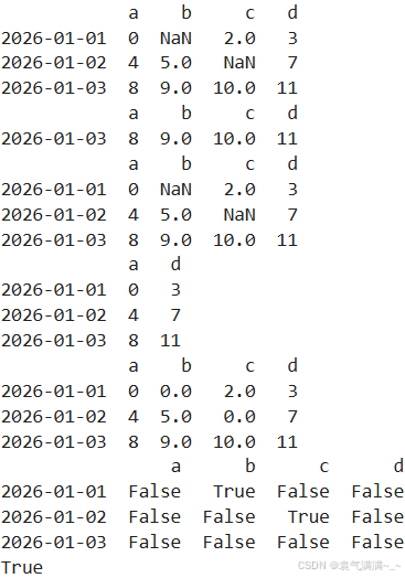
pd.read_csv():从 CSV 文件读取数据并加载为 DataFrame
DataFrame.to_csv():将 DataFrame 写入到 CSV 文件
pd.read_excel():读取 Excel 文件,返回 DataFrame
DataFrame.to_excel():将 DataFrame 写入 Excel 文件
python
data = pd.read_csv("student.csv")
print(data)
data.to_pickle("student.pickle")
pd.concat():沿指定轴将多个DataFrame或Series对象连接起来
DataFrame._append():将一行或多行附加到DataFrame的末尾
python
df1 = pd.DataFrame(np.zeros((3,4)),columns=['a','b','c','d'])
df2 = pd.DataFrame(np.ones((3,4)),columns=['a','b','c','d'])
df3 = pd.DataFrame(np.ones((3,4))*2,columns=['a','b','c','d'])
res = pd.concat([df1,df2,df3],axis=0,ignore_index=True)
print(res)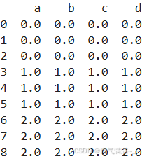
python
df1 = pd.DataFrame(np.zeros((3,4)),columns=['a','b','c','d'],index=[1,2,3])
df2 = pd.DataFrame(np.ones((3,4)),columns=['b','c','d','e'],index=[2,3,4])
res1 = pd.concat([df1,df2],join='outer')
print(res1)
res2 = pd.concat([df1,df2],join='inner',ignore_index=True)
print(res2)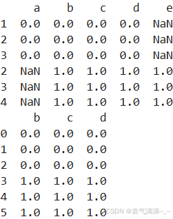
python
df1 = pd.DataFrame(np.zeros((3,4)),columns=['a','b','c','d'])
df2 = pd.DataFrame(np.ones((3,4)),columns=['a','b','c','d'])
df3 = pd.DataFrame(np.ones((3,4))*2,columns=['a','b','c','d'])
res = df1._append([df2,df3],ignore_index=True)
print(res)
s1 = pd.Series([1,2,3,4],index=['a','b','c','d'])
res = df1._append(s1,ignore_index=True)
print(res)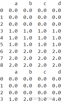
pd.merge():合并DataFrame或Series对象
- left:拼接的左侧DataFrame对象
- right:拼接的右侧DataFrame对象
- on:确定哪个字段作为主键
- how:包含'left', 'right', 'outer', 'inner',默认inner。inner是取交集,outer取并集
- indicator:将一列添加到名为_merge的输出DataFrame,显示拼接后的表中哪些信息来自于哪一个表格
- left_index:如果为True,则使用左侧DataFrame中的索引(行标签)作为其连接键
- right_index:与left_index相似
- suffixes:拼接后的表中有相同的列名(eg:age),且每列会有一个后缀(默认是age_x和age_y)表示这个列来自于哪个表格,通过修改参数suffixes='_boys','_girls',后缀变为age_boys和age_girls
python
left = pd.DataFrame({'Key':['k0','k1','k2','k3'],
                     'Key1':['k0','k1','k1','k2'],
                     'A':['a0','a1','a2','a3'],
                     'B':['b0','b1','b2','b3']})
right = pd.DataFrame({'Key':['k0','k11','k2','k3'],
                      'Key1':['k0','k2','k2','k2'],
                     'C':['c0','c1','c2','c3'],
                     'D':['d0','d1','d2','d3']})
res = pd.merge(left,right,on=['Key','Key1']) # pd.merge(left,right,on=['Key','Key1'],how='inner')
print(res)
res = pd.merge(left,right,on=['Key','Key1'],how='outer',indicator=True)
print(res)
res = pd.merge(left,right,on=['Key','Key1'],how='right')
print(res)
res = pd.merge(left,right,on=['Key','Key1'],how='left',indicator='indicator_column')
print(res)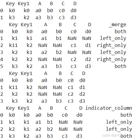
python
left = pd.DataFrame({'A':['a0','a1','a2','a3'],
                     'B':['b0','b1','b2','b3']},
                   index=['k0','k1','k2','k3'])
right = pd.DataFrame({'C':['c0','c1','c2','c3'],
                     'D':['d0','d1','d2','d3']},
                    index=['k1','k2','k3','k4'])
res = pd.merge(left,right,left_index=True,right_index=True,how='outer')
print(res)
res = pd.merge(left,right,left_index=True,right_index=True,how='inner')
print(res)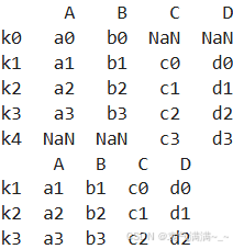
python
boys = pd.DataFrame({'k':['k0','k1','k2'],'age':[1,2,3]})
girls = pd.DataFrame({'k':['k0','k0','k3'],'age':[4,5,6]})
res = pd.merge(boys,girls,on='k',suffixes=['_boys','_girls'],how='inner')
print(res)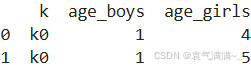
DataFrame.join():将两个或多个DataFrame或Series对象按照索引(行标签)或者某个特定的列进行连接。默认情况下,join() 方法使用的是左连接(left join),即以调用方法的 DataFrame 的索引为基准
python
df1 = pd.DataFrame({'A': ['A0', 'A1', 'A2'],
                   'B': ['B0', 'B1', 'B2']},
                  index=['K0', 'K1', 'K2'])
df2 = pd.DataFrame({'C': ['C0', 'C2', 'C3'],
                   'D': ['D0', 'D2', 'D3']},
                  index=['K0', 'K2', 'K3'])
res = df1.join(df2)
print(res)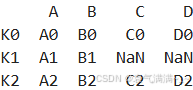
三、Matplotlib
python
import matplotlib.pyplot as plt
python
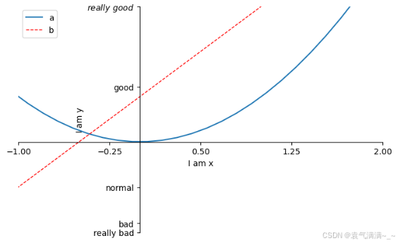
x = np.linspace(-3,3,50)
y1 = 2*x+1
y2 = x**2

plt.figure()
plt.plot(x,y1)


plt.figure(num=3,figsize=(8,5))
l1, = plt.plot(x,y2,label='up')
l2, = plt.plot(x,y1,color='red',linewidth=1,linestyle='--',label='down')

plt.legend(handles=[l1,l2],labels=['a','b'],loc='best')

plt.xlim(-1,2) # x轴取值范围
plt.ylim(-2,3) # y轴取值范围

plt.xlabel('I am x')
plt.ylabel('I am y')

new_ticks = np.linspace(-1,2,5) # [-1.   -0.25  0.5   1.25  2.  ]
plt.xticks(new_ticks)
plt.yticks([-2,-1.8,-1,1.22,3],
           ['really bad','bad','normal','good',r'$really\ good$']) # 通过r'$...$'可以使字体更美观

ax = plt.gca()
ax.spines['right'].set_color('none')
ax.spines['top'].set_color('none')
ax.xaxis.set_ticks_position('bottom')
ax.yaxis.set_ticks_position('left')
ax.spines['bottom'].set_position(('data',0))
ax.spines['left'].set_position(('data',0))

plt.show()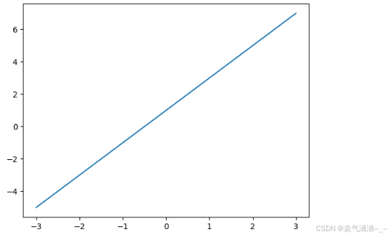
python
x = np.linspace(-3,3,50)
y = 2*x+1

plt.figure()
plt.plot(x,y)

ax = plt.gca()
ax.spines['right'].set_color('none')
ax.spines['top'].set_color('none')
ax.xaxis.set_ticks_position('bottom')
ax.yaxis.set_ticks_position('left')
ax.spines['bottom'].set_position(('data',0))
ax.spines['left'].set_position(('data',0))

x0 = 1
y0 = 2*x0+1
plt.scatter(x0,y0,s=50,color='r')
plt.plot([x0,x0],[y0,0],'k--',lw=2.5)

plt.annotate(r'$2x+1=%s$' % y0,xy=(x0,y0),xycoords='data',xytext=(+30,-30),textcoords='offset points',
             fontsize=16,arrowprops=dict(arrowstyle='->',connectionstyle='arc3,rad=.2'))

plt.text(-3,3,r'$This\ is\ text.\mu\ \sigma_i\ \alpha_t$',fontdict={'size':16,'color':'r'})

plt.show()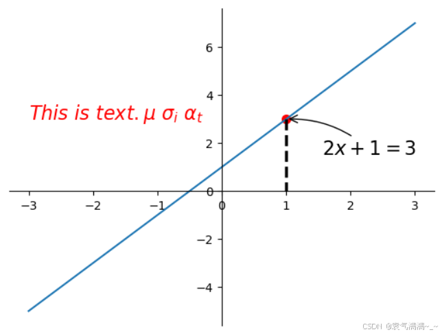
python
x = np.linspace(-3,3,50)
y = 0.1*x

plt.figure()
plt.plot(x,y,linewidth=10,zorder=1)
plt.ylim(-2,2)

ax = plt.gca()
ax.spines['right'].set_color('none')
ax.spines['top'].set_color('none')
ax.xaxis.set_ticks_position('bottom')
ax.yaxis.set_ticks_position('left')
ax.spines['bottom'].set_position(('data',0))
ax.spines['left'].set_position(('data',0))

for label in ax.get_xticklabels()+ax.get_yticklabels():
    label.set_fontsize(12)
    label.set_bbox(dict(facecolor='grey',edgecolor='None',alpha=0.7))


plt.show()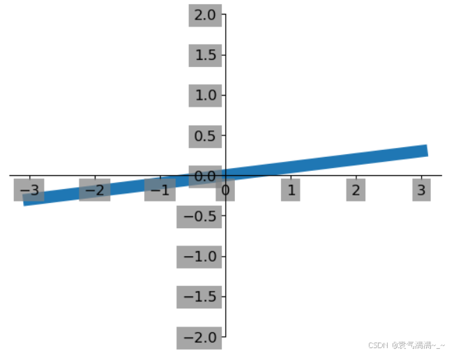
python
n = 1024
x = np.random.normal(0,1,n)
y = np.random.normal(0,1,n)
T = np.arctan2(y,x)

plt.scatter(x,y,s=75,c=T,alpha=0.5)

plt.xlim(-1.5,1.5)
plt.ylim(-1.5,1.5)
plt.xticks(())
plt.yticks(())

plt.show()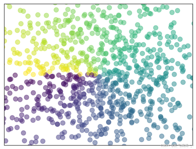
python
n = 12
x = np.arange(n)
y1 = (1-x/float(n))*np.random.uniform(0.5,1.0,n)
y2 = (1-x/float(n))*np.random.uniform(0.5,1.0,n)

plt.bar(x,+y1,facecolor='#9999ff',edgecolor='white')
plt.bar(x,-y2,facecolor='#ff9999',edgecolor='white')

for i,j in zip(x,y1):
    plt.text(i,j+0.05,'%.2f' % j,ha='center',va='bottom') # ha:horizontal alignment

for i,j in zip(x,y2):
    plt.text(i,-j-0.05,'-%.2f' % j,ha='center',va='top')

plt.xlim(-.5,n)
plt.ylim(-1.25,1.25)
plt.xticks(())
plt.yticks(())
plt.show()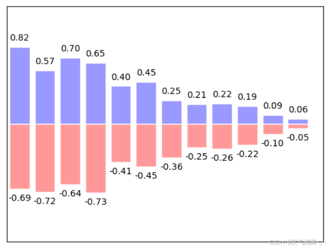
python
def f(x,y):
    return (1-x/2+x**5+y**3)*np.exp(-x**2-y**2)

n = 256
x = np.linspace(-3,3,n)
y = np.linspace(-3,3,n)

X,Y = np.meshgrid(x,y)

plt.contourf(X,Y,f(X,Y),8,alpha=0.75,cmap=plt.cm.hot)

C = plt.contour(X,Y,f(X,Y),8,colors='black',linewidths=.5)

plt.clabel(C,inline=True,fontsize=10)

plt.xticks(())
plt.yticks(())
plt.show()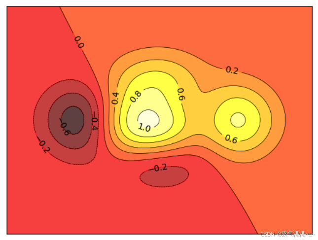
python
a = np.array([0.314,0.365,0.424,
              0.365,0.440,0.525,
             0.424,0.525,0.652]).reshape(3,3)

plt.imshow(a,interpolation='nearest',cmap='bone',origin='upper')
plt.colorbar(shrink=0.9) # 不设置shrink的颜色条长度与图片等高

plt.xticks(())
plt.yticks(())
plt.show()
python
from mpl_toolkits.mplot3d import Axes3D

fig = plt.figure()
ax = Axes3D(fig)

X = np.arange(-4,4,0.25)
Y = np.arange(-4,4,0.25)
X,Y = np.meshgrid(X,Y)
R = np.sqrt(X**2+Y**2)
Z = np.sin(R)

ax.plot_surface(X,Y,Z,rstride=1,cstride=1,cmap=plt.get_cmap('rainbow'),edgecolor='k')
ax.contourf(X,Y,Z,zdir='z',offset=-2,cmap='rainbow')
ax.set_zlim(-2,2)

fig.add_axes(ax)
plt.show()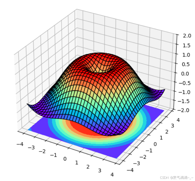
python
plt.figure()
plt.subplot(2,1,1)  # 2行1列
plt.plot([0,1],[0,1])

plt.subplot(234)  #
plt.plot([0,1],[0,2])

plt.subplot(2,3,5)
plt.plot([0,1],[0,3])

plt.subplot(2,3,6)
plt.plot([0,1],[0,4])

plt.show()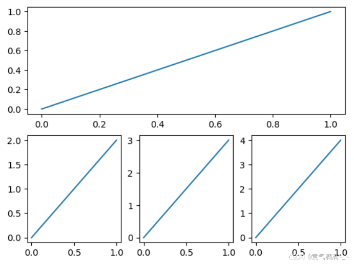
python
import matplotlib.gridspec as gridspec

plt.figure()

# 方法一
ax1 = plt.subplot2grid((3,3),(0,0),colspan=3,rowspan=1)
ax1.plot([1,2],[1,2])
ax1.set_title('ax1_title')
ax2 = plt.subplot2grid((3,3),(1,0),colspan=2,rowspan=1)
ax3 = plt.subplot2grid((3,3),(1,2),colspan=1,rowspan=2)
ax4 = plt.subplot2grid((3,3),(2,0),colspan=1,rowspan=1)
ax5 = plt.subplot2grid((3,3),(2,1),colspan=1,rowspan=1)


#方法二
gs = gridspec.GridSpec(3,3)
ax1 = plt.subplot(gs[0,:])
ax1.plot([1,2],[1,2])
ax1.set_title('ax1_title')
ax2 = plt.subplot(gs[1,:2])
ax3 = plt.subplot(gs[1:,2])
ax4 = plt.subplot(gs[-1,0])
ax5 = plt.subplot(gs[-1,-2])


plt.show()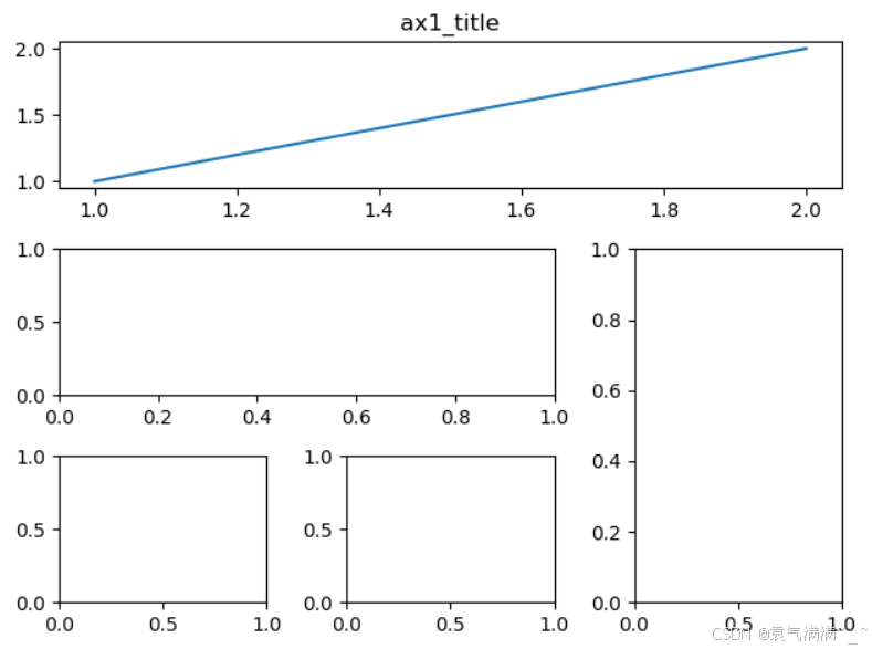
python
f, ((ax11, ax12), (ax21, ax22)) = plt.subplots(2, 2, sharex=True, sharey=True)

ax11.plot([1, 2], [1, 2])
ax11.set_title('ax1_title')

plt.show()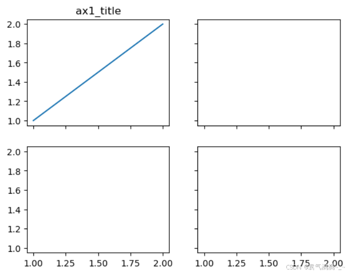
python
fig = plt.figure()
x = [1,2,3,4,5,6,7]
y = [1,3,4,2,5,8,6]

left,bottom,width,height = 0.1,0.1,0.8,0.8
ax1 = fig.add_axes([left,bottom,width,height])
ax1.plot(x,y,'r')
ax1.set_xlabel('x')
ax1.set_ylabel('y')
ax1.set_title('title')

left,bottom,width,height = 0.2,0.6,0.25,0.25
ax2 = fig.add_axes([left,bottom,width,height])
ax2.plot(y,x,'b')
ax2.set_xlabel('x')
ax2.set_ylabel('y')
ax2.set_title('inside one')

plt.axes([.6,.2,.25,.25])
plt.plot(y[::-1],x,'g')
plt.xlabel('x')
plt.ylabel('y')
plt.title('inside two')

plt.show()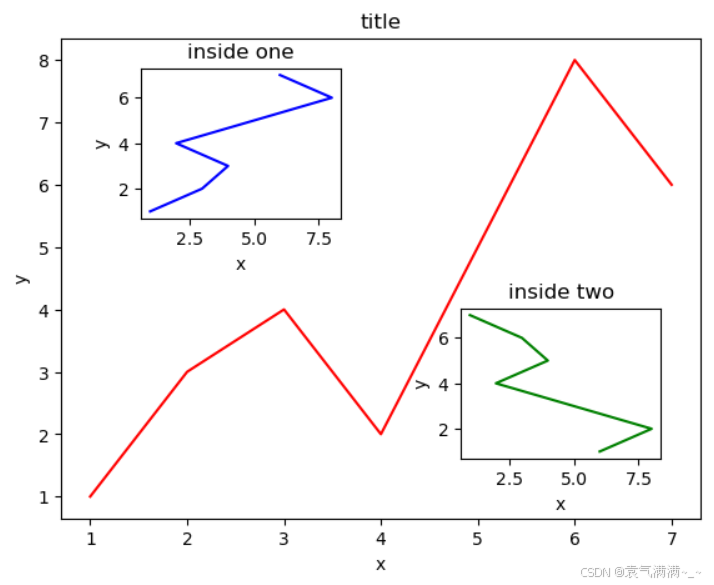
python
x = np.arange(0,10,0.1)
y1 = 0.05*x**2
y2 = -1*y1
fig,ax1 = plt.subplots()
ax2 = ax1.twinx()
ax1.plot(x,y1,'g-')
ax2.plot(x,y2,'b--')

ax1.set_xlabel('x_data')
ax1.set_ylabel('y1',color='g')
ax2.set_ylabel('y2',color='b')

plt.show()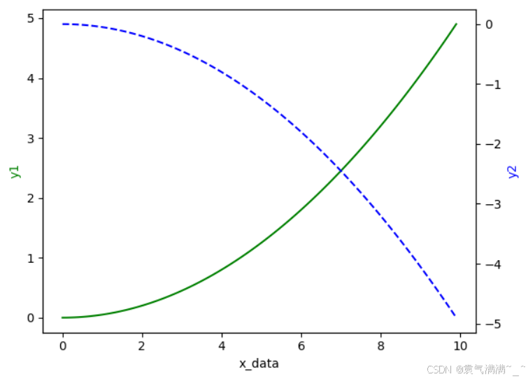
python
import matplotlib.pyplot as plt
import numpy as np

from matplotlib import animation

fig,ax = plt.subplots()

x = np.arange(0,2*np.pi,0.01)
line, = ax.plot(x,np.sin(x))

def animate(i):
    line.set_ydata(np.sin(x+i/10))
    return line,

def init():
    line.set_ydata(np.sin(x))
    return line,

ani = animation.FuncAnimation(fig=fig,func=animate,frames=100,init_func=init,interval=20,blit=True)

plt.show()

# 如果在pycharm中运行未显示动图,可通过setting->Tools->Python Plots把Show plots in tool window的勾去掉来解决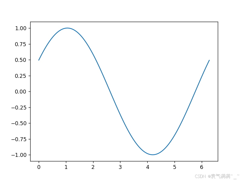
四、练习
数据:下载
- 获取 2020 年 2 月 3 日的所有数据
- 2020 年 1 月 24 日之前的累积确诊病例有多少个?
- 2020 年 7 月 23 日的新增死亡数是多少?
- 从 1 月 25 日到 7 月 22 日,一共增长了多少确诊病例?
- 每天新增确诊数和新恢复数的比例?平均比例,标准差各是多少?
- 画图展示新增确诊的变化曲线
- 画图展示死亡率的变化曲线
我主要用的是pandas方法来处理数据的,使用numpy方法的看这里。
python
import numpy as np
import pandas as pd
import matplotlib.pyplot as plt

# 获取2020年2月3日的所有数据
data = pd.read_csv('covid19_day_wise.csv',index_col='Date')
#print(data)
print(data.loc['2020-02-03'])

# 截至2020年1月24日累计确诊多少
print('-->截至2020年1月24日累计确诊:',data.loc['2020-01-24']['Confirmed'])

# 2020年7月23日的新增死亡人数是多少
print('-->2020年7月23日的新增死亡人数:',data.loc['2020-07-23']['New deaths'])

# 从1月25日到7月22日,一共新增多少确诊病例
print('-->期间共增长了:',np.sum(data.loc['2020-01-26':'2020-07-22','New cases']))

# 每天新增确诊数和新恢复数的比例?平均比例,标准差各是多少?
no_zero_mask = (data.loc[:,'New recovered']!=0)
r = data.loc[:,'New cases'] / data.loc[:,'New recovered']
print('平均比例:', np.mean(r) , '\n标准差:' , np.std(r))

# 画图展示新增确诊的变化曲线
#data.loc[:,'New cases'].plot()
x = data.index
plt.subplot(1,2,1)
plt.plot(x,data.loc[:,'New cases'])
plt.xticks(())

# 画图展示死亡率的变化曲线
#data.loc[:,'Deaths / 100 Cases'].plot()
plt.subplot(1,2,2)
plt.plot(x,data.loc[:,'Deaths / 100 Cases'])
plt.xticks(())
plt.show()