import torch
import torch.nn as nn
# 定义简单的线性模型(无隐藏层)
# 输入2个纬度的数据,得到1个纬度的输出
class SimpleNet(nn.Module):
def __init__(self):
super(SimpleNet, self).__init__()
# 线性层:2个输入特征,1个输出特征
self.linear = nn.Linear(2, 1)
def forward(self, x):
# 前向传播:y = w1*x1 + w2*x2 + b
return self.linear(x)
# 创建模型实例
model = SimpleNet()
# 查看模型参数
print("模型参数:")
for name, param in model.named_parameters():
print(f"{name}: {param.data}")
import torch
import torch.nn as nn
import matplotlib.pyplot as plt
import numpy as np
# 设置设备
device = torch.device("cuda:0" if torch.cuda.is_available() else "cpu")
# 定义极简CNN模型(仅1个卷积层+1个全连接层)
class SimpleCNN(nn.Module):
def __init__(self):
super(SimpleCNN, self).__init__()
# 卷积层:输入3通道,输出16通道,卷积核3x3
self.conv1 = nn.Conv2d(3, 16, kernel_size=3, padding=1)
# 池化层:2x2窗口,尺寸减半
self.pool = nn.MaxPool2d(kernel_size=2)
# 全连接层:展平后连接到10个输出(对应10个类别)
# 输入尺寸:16通道 × 16x16特征图 = 16×16×16=4096
self.fc = nn.Linear(16 * 16 * 16, 10)
def forward(self, x):
# 卷积+池化
x = self.pool(self.conv1(x)) # 输出尺寸: [batch, 16, 16, 16]
# 展平
x = x.view(-1, 16 * 16 * 16) # 展平为: [batch, 4096]
# 全连接
x = self.fc(x) # 输出尺寸: [batch, 10]
return x
# 初始化模型
model = SimpleCNN()
model = model.to(device)
# 查看模型结构
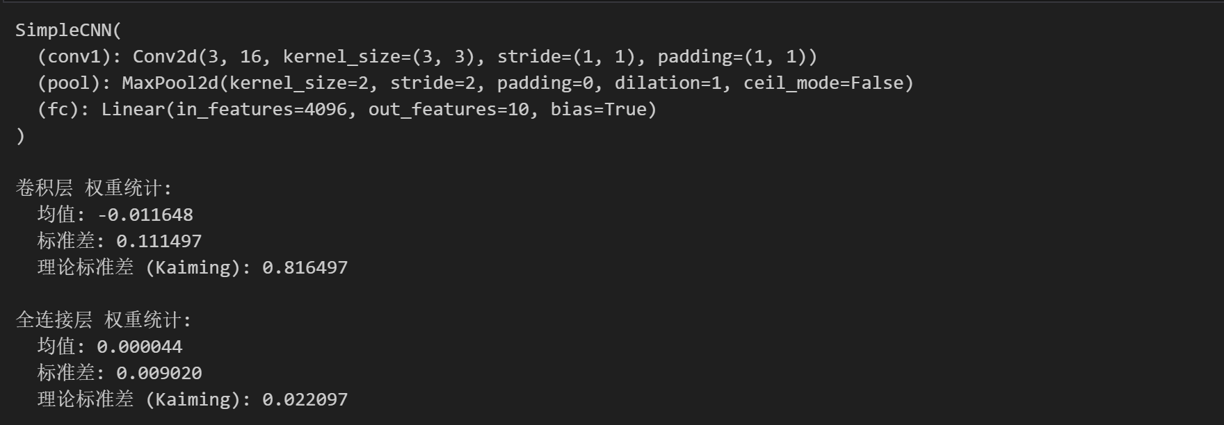
print(model)
# 查看初始权重统计信息
def print_weight_stats(model):
# 卷积层
conv_weights = model.conv1.weight.data
print("\n卷积层 权重统计:")
print(f" 均值: {conv_weights.mean().item():.6f}")
print(f" 标准差: {conv_weights.std().item():.6f}")
print(f" 理论标准差 (Kaiming): {np.sqrt(2/3):.6f}") # 输入通道数为3
# 全连接层
fc_weights = model.fc.weight.data
print("\n全连接层 权重统计:")
print(f" 均值: {fc_weights.mean().item():.6f}")
print(f" 标准差: {fc_weights.std().item():.6f}")
print(f" 理论标准差 (Kaiming): {np.sqrt(2/(16*16*16)):.6f}")
# 改进的可视化权重分布函数
def visualize_weights(model, layer_name, weights, save_path=None):
plt.figure(figsize=(12, 5))
# 权重直方图
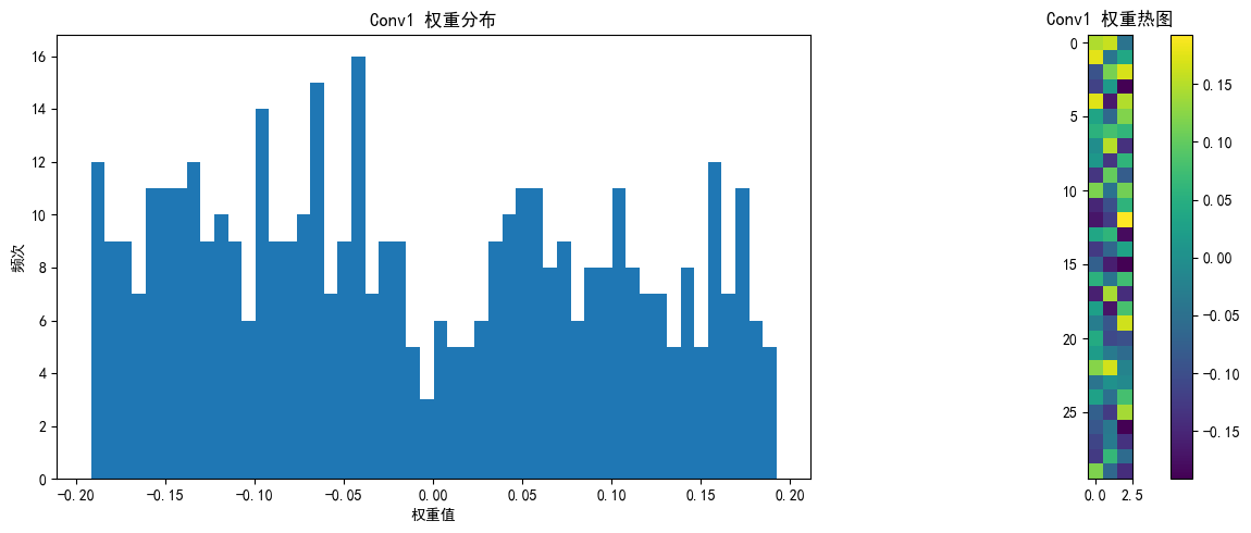
plt.subplot(1, 2, 1)
plt.hist(weights.cpu().numpy().flatten(), bins=50)
plt.title(f'{layer_name} 权重分布')
plt.xlabel('权重值')
plt.ylabel('频次')
# 权重热图
plt.subplot(1, 2, 2)
if len(weights.shape) == 4: # 卷积层权重 [out_channels, in_channels, kernel_size, kernel_size]
# 只显示第一个输入通道的前10个滤波器
w = weights[:10, 0].cpu().numpy()
plt.imshow(w.reshape(-1, weights.shape[2]), cmap='viridis')
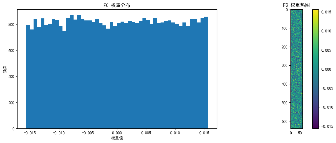
else: # 全连接层权重 [out_features, in_features]
# 只显示前10个神经元的权重,重塑为更合理的矩形
w = weights[:10].cpu().numpy()
# 计算更合理的二维形状(尝试接近正方形)
n_features = w.shape[1]
side_length = int(np.sqrt(n_features))
# 如果不能完美整除,添加零填充使能重塑
if n_features % side_length != 0:
new_size = (side_length + 1) * side_length
w_padded = np.zeros((w.shape[0], new_size))
w_padded[:, :n_features] = w
w = w_padded
# 重塑并显示
plt.imshow(w.reshape(w.shape[0] * side_length, -1), cmap='viridis')
plt.colorbar()
plt.title(f'{layer_name} 权重热图')
plt.tight_layout()
if save_path:
plt.savefig(f'{save_path}_{layer_name}.png')
plt.show()
# 打印权重统计
print_weight_stats(model)
# 可视化各层权重
visualize_weights(model, "Conv1", model.conv1.weight.data, "initial_weights")
visualize_weights(model, "FC", model.fc.weight.data, "initial_weights")
# 可视化偏置
plt.figure(figsize=(12, 5))
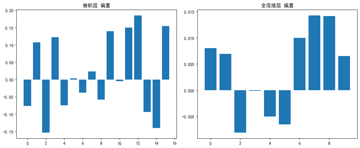
# 卷积层偏置
conv_bias = model.conv1.bias.data
plt.subplot(1, 2, 1)
plt.bar(range(len(conv_bias)), conv_bias.cpu().numpy())
plt.title('卷积层 偏置')
# 全连接层偏置
fc_bias = model.fc.bias.data
plt.subplot(1, 2, 2)
plt.bar(range(len(fc_bias)), fc_bias.cpu().numpy())
plt.title('全连接层 偏置')
plt.tight_layout()
plt.savefig('biases_initial.png')
plt.show()
print("\n偏置统计:")
print(f"卷积层偏置 均值: {conv_bias.mean().item():.6f}")
print(f"卷积层偏置 标准差: {conv_bias.std().item():.6f}")
print(f"全连接层偏置 均值: {fc_bias.mean().item():.6f}")
print(f"全连接层偏置 标准差: {fc_bias.std().item():.6f}")