opencv计算机视觉--图形透视(投影)变换&图形拼接

一、图形透视(投影)变换

1、什么是透视变换？

透视变换 是一种将图像从一个视角投影到另一个视角的几何变换，也称为投影变换 或单应性变换 。它模拟了真实世界中近大远小的透视效果。

生活中的例子：

1. 拍照时：倾斜拍书本，文字会变形

2. 看风景时：远处的山看起来比近处的树小

3. 文档扫描：手机倾斜拍摄的发票需要校正

2、代码中的透视变换实现

1） order_points(pts) - 点排序函数

def order_points(pts):
    rect = np.zeros((4, 2), dtype="float32")
    s = pts.sum(axis=1)  # 计算每个点的x+y
    rect[0] = pts[np.argmin(s)]   # 左上点：x+y最小
    rect[2] = pts[np.argmax(s)]   # 右下点：x+y最大
    
    diff = np.diff(pts, axis=1)   # 计算每个点的x-y
    rect[1] = pts[np.argmin(diff)]  # 右上点：x-y最小
    rect[3] = pts[np.argmax(diff)]  # 左下点：x-y最大
    
    return rect  # 返回排序后的点：[左上, 右上, 右下, 左下]

为什么要排序？

• 原始检测到的四个点是乱序的

• 透视变换需要知道点的对应关系

• 必须明确：源图像的左上角对应目标图像的左上角

2）four_point_transform() - 透视变换主函数

这是最核心的部分，我们一步步分解：

步骤1：获取排序后的点

rect = order_points(pts)  # 排序四个点
(tl, tr, br, bl) = rect   # 解包：左上、右上、右下、左下

步骤2：计算新图像的宽度

# 计算底边宽度（右下到左下）
widthA = np.sqrt(((br[0] - bl[0]) ** 2) + ((br[1] - bl[1]) ** 2))

# 计算顶边宽度（右上到左上）
widthB = np.sqrt(((tr[0] - tl[0]) ** 2) + ((tr[1] - tl[1]) ** 2))

# 取最大值作为新宽度
maxWidth = max(int(widthA), int(widthB))

为什么取最大值？

• 确保新图像能完整包含原始内容

• 避免裁剪

步骤3：计算新图像的高度

# 计算右边高度（右上到右下）
heightA = np.sqrt(((tr[0] - br[0]) ** 2) + ((tr[1] - br[1]) ** 2))

# 计算左边高度（左上到左下）
heightB = np.sqrt(((tl[0] - bl[0]) ** 2) + ((tl[1] - bl[1]) ** 2))

# 取最大值作为新高度
maxHeight = max(int(heightA), int(heightB))

步骤4：定义目标点（校正后的矩形）

dst = np.array([
    [0, 0],                    # 左上：坐标原点
    [maxWidth - 1, 0],         # 右上：最右列，最上行
    [maxWidth - 1, maxHeight - 1],  # 右下：最右列，最下行
    [0, maxHeight - 1]         # 左下：最左列，最下行
], dtype="float32")

步骤5：计算透视变换矩阵（关键！）

M = cv2.getPerspectiveTransform(rect, dst)

这个函数做了什么？

• 输入：4对对应点（源点rect，目标点dst）

• 输出：3×3的变换矩阵M

• 数学上：解一个线性方程组，找到变换参数

步骤6：应用透视变换（关键！）

warped = cv2.warpPerspective(image, M, (maxWidth, maxHeight))

这个函数做了什么？

• 对图像中每个像素应用变换矩阵M

• 进行插值计算，得到新图像

• 输出尺寸为(maxWidth, maxHeight)

3.实际运用（发票扫描与校正）

这是一个完整的发票/文档扫描与校正程序，实现了从倾斜拍摄的发票到正面校正图像的全流程处理。

1）程序总体流程

读取图像 → 预处理 → 轮廓检测 → 文档定位 → 透视变换 → 后处理

2）详细步骤解析

第1部分：图像预处理

1. 定义工具函数

def cv_show(name, img):  # 显示图像
def resize(image, width=None, height=None):  # 保持比例调整大小

2. 读取和缩放图像

image = cv2.imread('fapiao.jpg')  # 读取发票图片
ratio = image.shape[0] / 500.0    # 计算缩放比例（原高/500）
orig = image.copy()               # 备份原始图像
image = resize(orig, height=500)  # 高度固定为500像素

目的 ：大图像处理慢，缩小可提高速度，记住ratio用于后续坐标转换。

第2部分：文档轮廓检测

1. 转换为灰度图

gray = cv2.cvtColor(image, cv2.COLOR_BGR2GRAY)

2. 边缘检测与二值化

edged = cv2.threshold(gray, 0, 255, cv2.THRESH_BINARY | cv2.THRESH_OTSU)[1]

OTSU算法：自动计算最佳阈值，适应不同光照条件。

3. 查找所有轮廓

cnts = cv2.findContours(edged.copy(), cv2.RETR_LIST, cv2.CHAIN_APPROX_SIMPLE)[-2]

• RETR_LIST：获取所有轮廓

• CHAIN_APPROX_SIMPLE：压缩轮廓点

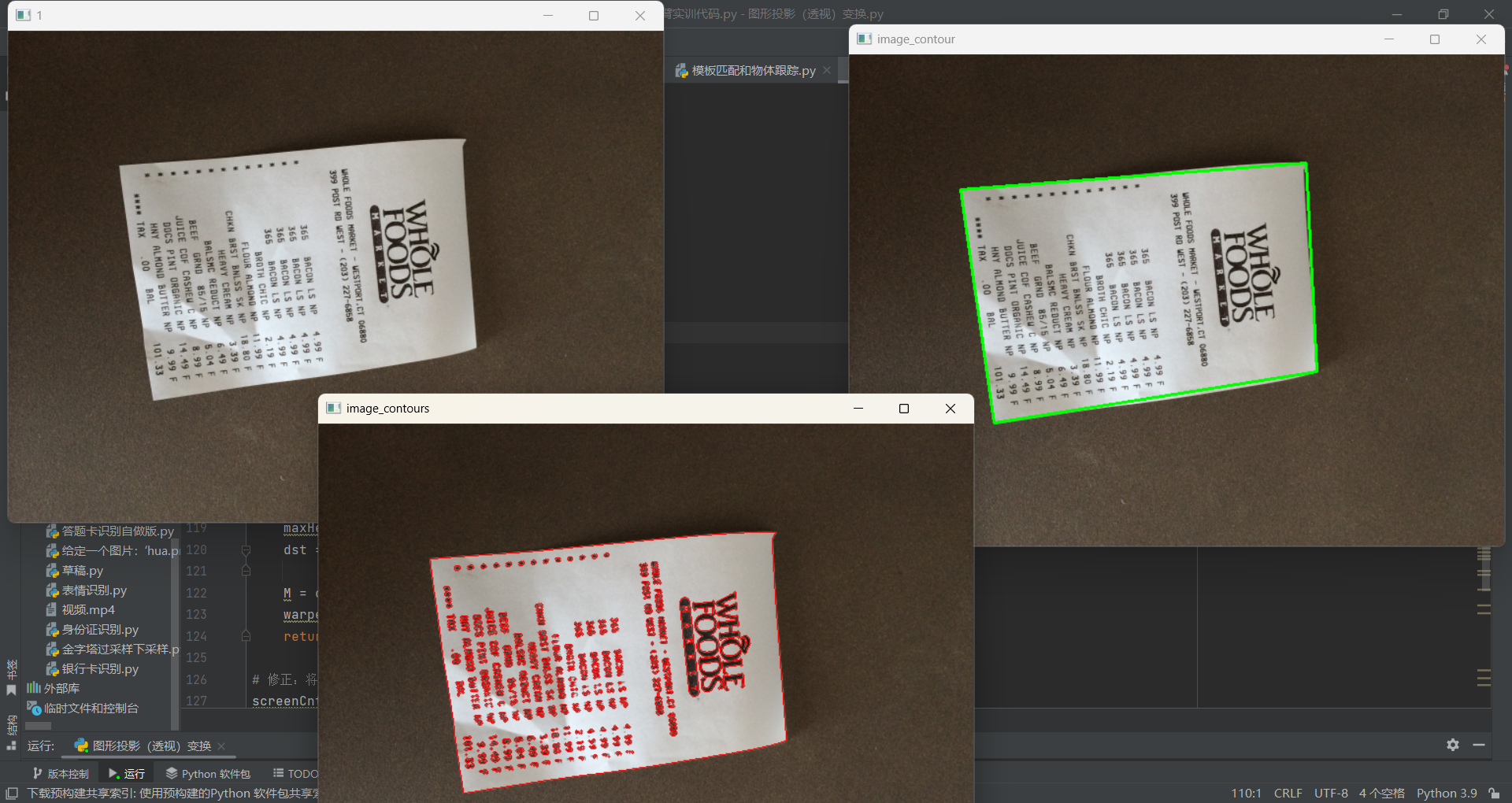
4. 可视化所有轮廓

image_contours = cv2.drawContours(image.copy(), cnts, -1, (0, 0, 255), 1)

第3部分：文档定位

1. 找到最大轮廓（假设文档最大）

screenCnt = sorted(cnts, key=cv2.contourArea, reverse=True)[0]

2. 轮廓多边形近似

peri = cv2.arcLength(screenCnt, True)  # 计算周长
screenCnt = cv2.approxPolyDP(screenCnt, 0.05 * peri, True)  # 近似为多边形

approxPolyDP：将曲线轮廓近似为直线多边形，精度=周长的5%。

3. 绘制文档轮廓

image_contour = cv2.drawContours(image.copy(), [screenCnt], -1, (0, 255, 0), 2)

绿色粗线框出找到的文档边界。

第4部分：透视变换核心函数

1. 点排序函数 order_points()

def order_points(pts):
    # 将4个无序点排序为：左上、右上、右下、左下
    # 方法：计算x+y和x-y，根据大小关系确定位置

2. 透视变换主函数 four_point_transform()

def four_point_transform(image, pts):
    # 1. 排序点
    # 2. 计算新图像尺寸（取最大宽度和高度）
    # 3. 定义目标矩形
    # 4. 计算透视变换矩阵 cv2.getPerspectiveTransform()
    # 5. 应用变换 cv2.warpPerspective()

第5部分：应用透视变换

1. 坐标映射回原始尺寸

screenCnt_points = screenCnt.reshape(4, 2) * ratio

关键 ：screenCnt是在小图（高500px）上找到的点，需要乘ratio得到原图坐标。

2. 执行透视变换

warped = four_point_transform(orig, screenCnt_points)

输入原始大图和四个角点，输出校正后的矩形文档。

3. 调整大小便于显示

warped_resized = resize(warped, height=500)

第6部分：图像后处理

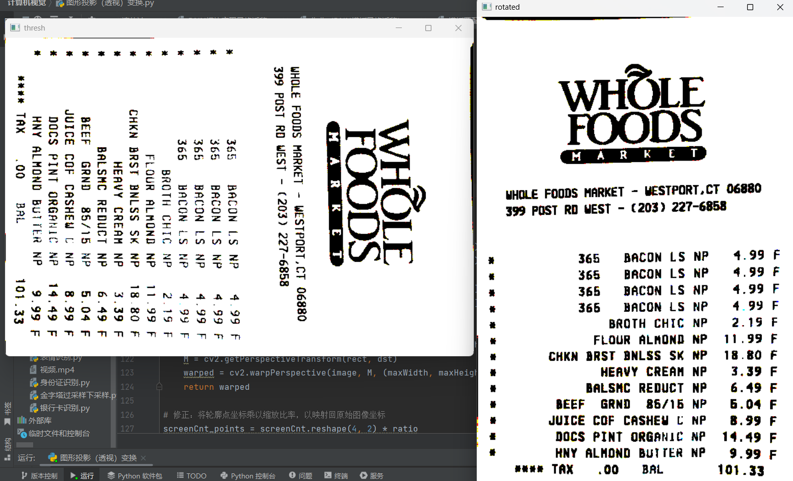
1. 二值化（黑白化）

thresh = cv2.threshold(warped_resized, 120, 255, cv2.THRESH_BINARY)[1]

阈值120：>120变白，≤120变黑，增强对比度。

2. 腐蚀去噪

kernel = np.ones((2, 2), np.uint8)
erode_1 = cv2.erode(thresh, kernel, iterations=1)

消除细小噪声，让文字更清晰。

3. 旋转校正

rotated = cv2.rotate(erode_1, cv2.ROTATE_90_COUNTERCLOCKWISE)

逆时针旋转90度，可能是因为原始发票是横向拍摄的。

完整代码部分

import numpy as np
import cv2

def cv_show(name, img):
    cv2.imshow(name, img)
    cv2.waitKey(0)
def resize(image,width=None,height=None,inter=cv2.INTER_AREA):
    dim=None
    (h,w)=image.shape[:2]
    if width is None and height is None:
        return image
    if width is None:
        r=height/float(h)
        dim=(int(w*r),height)
    else:
        r=width/float(w)
        dim=(width,int(h*r))
    resized=cv2.resize(image,dim,interpolation=inter)    #默认为cv2.INTER_AREA，即面积插值，适用于缩放图像。
    return resized
# 读取输入
image = cv2.imread('fapiao.jpg')
cv_show('image', image)

# 图片过大，进行缩小处理
ratio = image.shape[0] / 500.0  # 计算缩小比率
orig = image.copy()
image = resize(orig, height=500)
cv_show('1', image)

# 轮廓检测
print("STEP 1：轮廓检测")
gray = cv2.cvtColor(image, cv2.COLOR_BGR2GRAY)  # 读取灰度图

edged = cv2.threshold(gray, 0, 255, cv2.THRESH_BINARY | cv2.THRESH_OTSU)[1]  # 自动寻找阈值二值化
cnts = cv2.findContours(edged.copy(), cv2.RETR_LIST, cv2.CHAIN_APPROX_SIMPLE)[-2]
image_contours = cv2.drawContours(image.copy(), cnts, -1, (0, 0, 255), 1)
cv_show('image_contours', image_contours)

print("STEP 2：获取最大轮廓")
screenCnt = sorted(cnts, key=cv2.contourArea, reverse=True)[0]  # 获取面积最大的轮廓
print(screenCnt.shape)
peri = cv2.arcLength(screenCnt, True)  # 计算轮廓周长
screenCnt = cv2.approxPolyDP(screenCnt, 0.05 * peri, True)  # 轮廓近似
print(screenCnt.shape)
image_contour = cv2.drawContours(image.copy(), [screenCnt], -1, (0, 255, 0), 2)

cv2.imshow("image_contour", image_contour)
cv2.waitKey(0)
cv2.destroyAllWindows()
def order_points(pts):
    rect = np.zeros((4, 2), dtype="float32")
    s = pts.sum(axis=1)
    rect[0] = pts[np.argmin(s)]
    rect[2] = pts[np.argmax(s)]
    diff = np.diff(pts, axis=1)
    rect[1] = pts[np.argmin(diff)]
    rect[3] = pts[np.argmax(diff)]
    return rect

def four_point_transform(image, pts):
    rect = order_points(pts)
    (tl, tr, br, bl) = rect
    widthA = np.sqrt(((br[0] - bl[0]) ** 2) + ((br[1] - bl[1]) ** 2))
    widthB = np.sqrt(((tr[0] - tl[0]) ** 2) + ((tr[1] - tl[1]) ** 2))
    maxWidth = max(int(widthA), int(widthB))
    heightA = np.sqrt(((tr[0] - br[0]) ** 2) + ((tr[1] - br[1]) ** 2))
    heightB = np.sqrt(((tl[0] - bl[0]) ** 2) + ((tl[1] - bl[1]) ** 2))
    maxHeight = max(int(heightA), int(heightB))
    dst = np.array([[0, 0], [maxWidth - 1, 0],
                   [maxWidth - 1, maxHeight - 1], [0, maxHeight - 1]], dtype="float32")
    M = cv2.getPerspectiveTransform(rect, dst)
    warped = cv2.warpPerspective(image, M, (maxWidth, maxHeight))
    return warped

# 修正：将轮廓点坐标乘以缩放比率，以映射回原始图像坐标
screenCnt_points = screenCnt.reshape(4, 2) * ratio
warped = four_point_transform(orig, screenCnt_points)
warped_resized = resize(warped, height=500)

thresh=cv2.threshold(warped_resized,120,255,cv2.THRESH_BINARY)[1]

#腐蚀操作
kernel = np.ones((2, 2), np.uint8)  # 创建一个2x2的矩形结构元素
erode_1 = cv2.erode(thresh, kernel, iterations=1)
# 逆时针旋转90度
rotated = cv2.rotate(erode_1, cv2.ROTATE_90_COUNTERCLOCKWISE)

# 或者顺时针旋转90度
# rotated = cv2.rotate(image, cv2.ROTATE_90_CLOCKWISE)

# 旋转180度
# rotated = cv2.rotate(image, cv2.ROTATE_180)

# cv2.imwrite('invoice_new.jpg', warped_resized)
# cv_show('warped', warped_resized)
# cv_show('warped_resized', warped_resized)
cv_show('thresh',thresh)
cv2.waitKey(0)
cv_show('rotated',rotated)
cv2.waitKey(0)
cv2.destroyAllWindows()

运行结果

3）核心算法总结

步骤	关键函数	作用
预处理	cv2.resize()	调整尺寸
边缘检测	cv2.threshold(OTSU)	自动二值化
轮廓查找	cv2.findContours()	提取轮廓
轮廓近似	cv2.approxPolyDP()	多边形近似
透视变换	cv2.getPerspectiveTransform()	计算变换矩阵
图像变换	cv2.warpPerspective()	应用透视变换
后处理	cv2.erode(), cv2.rotate()	去噪和旋转

这是一个完整的、可实际使用的文档扫描系统，涵盖了计算机视觉中的多个关键技术：边缘检测、轮廓分析、几何变换、图像增强等。

二、图片拼接

1、cv2.findHomography()

这是图像拼接和计算机视觉中最核心的函数之一 ，用于计算两个平面之间的单应性变换矩阵（Homography Matrix）。

计算透视变换矩阵
findHomography(srcPoints, dstPoints, method=None, ransacReprojThreshold=None, mask=None, maxIters=None, confidence=None)
参数说明：
srcPoints: 原图像匹配点坐标（这里是图片B的特征点）
dstPoints: 目标图像匹配点坐标（这里是图片A的特征点）
method: 计算变换矩阵的方法：
  0 - 使用所有的点，最小二乘
  RANSAC - 基于随机样本一致性
  LMEDS - 最小中值
  RHO - 基于渐近样本一致性
ransacReprojThreshold: 最大允许重投影错误阈值（默认为3）
返回值：H为变换矩阵，mask为掩模标志，指示哪些点是内点/外点

2、参数详细说明

(H, mask) = cv2.findHomography(srcPoints, dstPoints, method=cv2.RANSAC, 
                               ransacReprojThreshold=3.0, maxIters=2000, 
                               confidence=0.995)

1） srcPoints - 源点

• 类型：np.array，形状为 (N, 1, 2) 或 (N, 2)

• 说明：第一幅图像中的特征点坐标

• 在你的代码中：ptsB（右图的特征点）

2.）dstPoints - 目标点

• 类型：np.array，形状为 (N, 1, 2) 或 (N, 2)

• 说明：第二幅图像中的对应特征点坐标

• 在你的代码中：ptsA（左图的特征点）

3）method - 计算方法（最重要！）

a) method=0 或 cv2.LMEDS

最小二乘法（使用所有点）

(H, _) = cv2.findHomography(ptsB, ptsA, 0)

• 原理：最小化所有点的重投影误差平方和

• 优点：数学上最优（无异常点时）

• 缺点：对异常点（错误匹配）非常敏感

• 适用：所有匹配点都准确的情况（罕见）

b) method=cv2.RANSAC ★ 最常用

随机采样一致性算法

(H, mask) = cv2.findHomography(ptsB, ptsA, cv2.RANSAC, ransacReprojThreshold=3.0)

• 原理：

  1. 随机选择4对点（最小样本集）

  2. 计算临时单应性矩阵

  3. 统计有多少点符合该矩阵（内点）

  4. 重复多次（如2000次），选择内点最多的模型

  5. 用所有内点重新计算精确矩阵

• 优点：对异常点（错误匹配）鲁棒

• 缺点：计算量稍大，结果具有随机性

• 你的代码中：使用了这个方法，阈值设为10（较宽松）

c) method=cv2.LMEDS

最小中值法

• 原理：最小化误差的中值

• 对异常点有一定鲁棒性，但不如RANSAC

d) method=cv2.RHO

渐进一致采样算法

• 原理：基于PROSAC改进，更高效

• 适用：当有很多匹配点时效率高

4） ransacReprojThreshold - RANSAC重投影阈值

• 默认值：3.0（像素）

• 你的代码：10.0（更宽松）

• 含义：一个点被认为是"内点"的最大允许误差

5）maxIters - 最大迭代次数

• 默认：2000

• RANSAC算法最多尝试的次数

• 更多迭代 → 更可能找到好模型，但更慢

6）confidence - 置信度

• 默认：0.995（99.5%）

• 表示算法至少找到一个只包含内点的样本的概率

• 更高置信度 → 更多迭代次数

3、总结

cv2.findHomography() 是计算机视觉中的基石函数：

1. 功能：计算两个视图之间的透视变换关系

2. 核心算法：RANSAC（处理错误匹配的关键）

3. 关键参数 ：ransacReprojThreshold（平衡严格与宽松）

4. 输出：变换矩阵H + 内点掩码mask

5. 应用：图像拼接、增强现实、相机标定、三维重建等

4、实际运用

右边图片进行透视变换，把左边图片拼接上去

import cv2
import numpy as np
import sys

def cv_show(name, img):
    """显示图像"""
    cv2.imshow(name, img)
    cv2.waitKey(0)

def detectAndDescribe(image):
    """检测图像特征点并计算描述符"""
    gray = cv2.cvtColor(image, cv2.COLOR_BGR2GRAY)  # 转为灰度图
    sift = cv2.SIFT_create()  # 创建SIFT检测器
    (kps, des) = sift.detectAndCompute(gray, None)  # 检测关键点并计算描述符
    kps_float = np.float32([kp.pt for kp in kps])  # 提取关键点坐标（浮点型）
    return (kps, kps_float, des)

# 读取图像
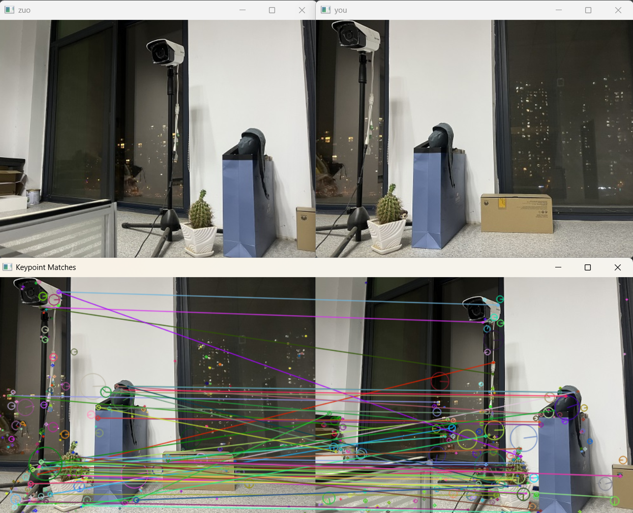
imageA = cv2.imread("zuo.jpg")
cv_show('zuo', imageA)
imageB = cv2.imread("you.jpg")
cv_show('you', imageB)

# 提取特征
(kpsA, kps_floatA, desA) = detectAndDescribe(imageA)
(kpsB, kps_floatB, desB) = detectAndDescribe(imageB)

# 使用暴力匹配器进行特征匹配
matcher = cv2.BFMatcher()
rawMatches = matcher.knnMatch(desB, desA, k=2)

# 筛选匹配对
good = []
matches = []
for m in rawMatches:
    if len(m) == 2 and m[0].distance < 0.65 * m[1].distance:
        good.append(m)
        matches.append((m[0].queryIdx, m[0].trainIdx))

print(f"匹配对数: {len(good)}")
print("匹配索引列表:", matches)


# 绘制匹配结果
vis = cv2.drawMatchesKnn(imageB, kpsB, imageA, kpsA, good,
                         outImg=None,
                         flags=cv2.DRAW_MATCHES_FLAGS_DRAW_RICH_KEYPOINTS)
cv_show("Keypoint Matches", vis)

# 透视变换
if len(matches) > 4:  # 当筛选后的匹配对大于4时，计算视角变换矩阵
    # 获取匹配对的点坐标
    # matches是通过阈值筛选之后的特征点对象
    # kps_floatA/kps_floatB是图片A/B中的全部特征点坐标
    ptsB = np.float32([kps_floatB[i] for (i, _) in matches])
    ptsA = np.float32([kps_floatA[i] for (_, i) in matches])

    # 计算透视变换矩阵
    (H, mask) = cv2.findHomography(ptsB, ptsA, cv2.RANSAC, ransacReprojThreshold=10)
else:
    print('图片未找到4个以上的匹配点')
    sys.exit()

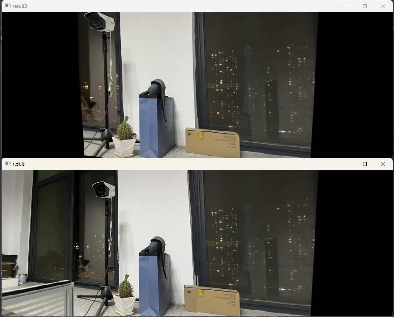
# 对图片B进行透视变换
# dsize参数指定输出图像大小：宽度为两图宽度之和，高度为图片B的高度
result = cv2.warpPerspective(imageB, H,
                             dsize=(imageB.shape[1] + imageA.shape[1], imageB.shape[0]))
cv_show('resultB', result)

# 将图片A拼接到结果图片的最左端
result[0:imageA.shape[0], 0:imageA.shape[1]] = imageA
cv_show('result', result)
cv2.destroyAllWindows()

运行结果