pytorch深度学习笔记19

目录

摘要

1.张量索引操作

2.张量形状操作

3.张量拼接操作

4.微分模块

5.机器学习案例：线性回归

---

摘要

本篇文章继续学习尚硅谷深度学习教程，学习内容是张量索引操作，形状操作，拼接操作，以及自动微分模块的实现和，学习线性回归的机器学习案例

1.张量索引操作

简单索引

import torch

tensor1 = torch.randint(1, 9, (3, 5, 4))
print(tensor1)
print()

# 取 第0维第0
print(tensor1[0])
print()

# 取 第0维所有，第1维第1
print(tensor1[:, 1])
print()

# 取 第0维所有，第1维第1，第2维第3
print(tensor1[2, 1, 3])

范围索引

import torch

tensor1 = torch.randint(1, 9, (3, 5, 4))
print(tensor1)
print()

# 取 第0维第1到最后
print(tensor1[1:])
print()

# 取 第0维最后，第1维1到3(包含3),第2维0到2(包含2)
print(tensor1[-1:, 1:4, 0:3])
print()

列表索引

import torch

tensor1 = torch.randint(1, 9, (3, 5, 4))
print(tensor1)
print()

# 取 第0维第0，第1维第1 和 第0维第1，第1维第2
print(tensor1[[0, 1], [1, 2]])
print()

# 取 第0维第0，第1维第1、2 和 第0维第1，第1维第1、2
print(tensor1[[[0], [1]], [1, 2]])

布尔索引

import torch

tensor1 = torch.randint(1, 9, (3, 5, 4))
print(tensor1)
print()

# 取 第2维第0大于5的，返回(dim0,dim1)形状的索引
print(tensor1[:, :, 0] > 5)
print(tensor1[tensor1[:, :, 0] > 5])
print()

# 取 第1维第1大于5的，返回(dim0,dim2)形状的索引
mask = tensor1[:, 1, :] > 5
print(mask)
tensor2 = tensor1.permute(0, 2, 1)  # 转换维度为(dim0,dim2,dim1)
print(tensor2[mask])
tensor2 = tensor2[mask].permute(1, 0)  # 转换维度为(dim1,?)
print(tensor2)
print()

# 取 第1维第1，第2维第2大于5的，返回(dim0)形状的索引
print(tensor1[:, 1, 2] > 5)
print(tensor1[tensor1[:, 1, 2] > 5])

2.张量形状操作

交换维度

transpose()交换两个维度， permute()重新排列多个维度

import torch

tensor1 = torch.randint(1, 9, (2, 3, 6))
print(tensor1)
print(tensor1.transpose(1, 2))  # 交换第1维和第2维

tensor1 = torch.randint(1, 9, (2, 3, 6))
print(tensor1)
print(tensor1.permute(2, 0, 1))  # (2, 3, 6)->(6, 2, 3)#重新排列

调整形状

reshape()调整张量的形状，view()调整张量的形状，需要内存连续。共享内存， is_contiguous()判断是否内存连续，contiguous()转换为内存连续

import torch

tensor1 = torch.randint(1, 9, (3, 5, 4))
print(tensor1)
print(tensor1.reshape(6, 10))
print(tensor1.reshape(3, -1))

tensor1 = torch.randint(1, 9, (3, 5, 4))
print(tensor1)
print(tensor1.is_contiguous())  # is_contiguous()判断是否内存连续
print(tensor1.view(-1, 10))

tensor1 = tensor1.T
print(tensor1.is_contiguous())  # is_contiguous()判断是否内存连续
print(tensor1.contiguous().view(-1))  # contiguous()强制内存连续

增加或删除维度

​​​​​​​unsqueeze()在指定维度上增加1个维度， ​​​​​​​squeeze()删除大小为1的维度

import torch

tensor1 = torch.tensor([1, 2, 3, 4, 5])
print(tensor1)
# 在0维上增加一个维度
print(tensor1.unsqueeze(dim=0))
# 在1维上增加一个维度
print(tensor1.unsqueeze(dim=1))
# 在-1维上增加一个维度
print(tensor1.unsqueeze(dim=-1))

tensor1 = torch.tensor([1, 2, 3, 4, 5])
print(tensor1.unsqueeze_(dim=0))
print(tensor1.squeeze())

3.张量拼接操作

​​​​​​​torch.cat()张量拼接，按已有维度拼接。除拼接维度外，其他维度大小须相同，torch.stack()张量堆叠，按新维度堆叠。所有张量形状必须一致

import torch

tensor1 = torch.randint(1, 9, (2, 2, 5))
tensor2 = torch.randint(1, 9, (2, 1, 5))
print(tensor1)
print(tensor2)
print(torch.cat([tensor1, tensor2], dim=1))

torch.manual_seed(42)
tensor1 = torch.randint(1, 9, (3, 1, 5))
tensor2 = torch.randint(1, 9, (3, 1, 5))
print(tensor1)
print(tensor2)
tensor3 = torch.stack([tensor1, tensor2], dim=2)
print(tensor3)
print(tensor3.shape)

4.微分模块

训练神经网络时，框架会根据设计好的模型构建一个计算图（computational graph），来跟踪计算是哪些数据通过哪些操作组合起来产生输出，并通过反向传播算法来根据给定参数的损失函数的梯度调整参数（模型权重）。

PyTorch具有一个内置的微分引擎torch.autograd以支持计算图的梯度自动计算。

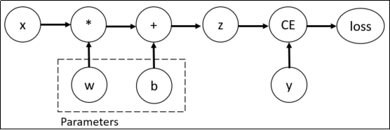
考虑最简单的单层神经网络，具有输入x、参数w、偏置b以及损失函数：

import torch

# 输入x
x = torch.tensor(10.0)
# 目标值y
y = torch.tensor(3.0)

# 初始化权重w
w = torch.rand(1, 1, requires_grad=True)
# 初始化偏置b
b = torch.rand(1, 1, requires_grad=True)
z = w * x + b
# 设置损失函数
loss = torch.nn.MSELoss()
loss_value = loss(z, y)
# 反向传播
loss_value.backward()
# 打印w,b的梯度
print("w的梯度:\n", w.grad)
print("b的梯度:\n", b.grad)

该计算图中x、w、b为叶子节点，即最基础的节点。叶子节点的数据并非由计算生成，因此是整个计算图的基石，叶子节点张量不可以执行in-place操作。而最终的loss为根节点。

可通过is_leaf属性查看张量是否为叶子节点：

print(x.is_leaf)  # True
print(w.is_leaf)  # True
print(b.is_leaf)  # True
print(z.is_leaf)  # False
print(y.is_leaf)  # True
print(loss_value.is_leaf)  # False

自动微分的关键就是记录节点的数据与运算。数据记录在张量的data属性中，计算记录在张量的grad_fn属性中。

计算图根据搭建方式可分为静态图和动态图，PyTorch是动态图机制，在计算的过程中逐步搭建计算图，同时对每个Tensor都存储grad_fn供自动微分使用。

若设置张量参数requires_grad=True，则PyTorch会追踪所有基于该张量的操作，并在反向传播时计算其梯度。依赖于叶子节点的节点，requires_grad默认为True。当计算到根节点后，在根节点调用backward()方法即可反向传播计算计算图中所有节点的梯度。

非叶子节点的梯度在反向传播之后会被释放掉（除非设置参数retain_grad=True）。而叶子节点的梯度在反向传播之后会保留（累积）。通常需要使用optimizer.zero_grad()清零参数的梯度。

有时我们希望将某些计算移动到计算图之外，可以使用Tensor.detach()返回一个新的变量，该变量与原变量具有相同的值，但丢失计算图中如何计算原变量的信息。换句话说，梯度不会在该变量处继续向下传播。例如：

import torch

x = torch.ones(2, 2, requires_grad=True)
y = x * x
# 分离y来返回一个新变量u
u = y.detach()
z = u * x
# 梯度不会向后流经u到x
z.sum().backward()
# 反向传播函数计算z=u*x关于x的偏导数时将u作为常数处理，而不是z=x*x*x关于x的偏导数
x.grad == u
# tensor([[True, True],
#         [True, True]])

5.机器学习案例：线性回归

通过PyTorch训练一个模型一般分为以下4个步骤：

准备数据 → 构建模型 → 定义损失函数与优化器 → 模型训练

接下来，构建数据集并使用PyTorch实现线性回归：

import torch
import matplotlib.pyplot as plt
from torch import nn, optim  # 模型、损失函数和优化器
from torch.utils.data import TensorDataset, DataLoader  # 数据集和数据加载器

# 构建数据集
X = torch.randn(100, 1)  # 输入
w = torch.tensor([2.5])  # 权重
b = torch.tensor([5.2])  # 偏置
noise = torch.randn(100, 1) * 0.1  # 噪声
y = w * X + b + noise  # 目标
dataset = TensorDataset(X, y)  # 构造数据集对象
dataloader = DataLoader(
    dataset, batch_size=10, shuffle=True
)  # 构造数据加载器对象，batch_size为每次训练的样本数，shuffle为是否打乱数据

# 构造模型
model = nn.Linear(in_features=1, out_features=1)  # 线性回归模型，1个输入，1个输出

# 损失函数和优化器
loss = nn.MSELoss()  # 均方误差损失函数
optimizer = optim.SGD(model.parameters(), lr=1e-3)  # 随机梯度下降，学习率0.001

# 模型训练
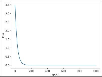
loss_list = []
for epoch in range(1000):
    total_loss = 0
    train_num = 0
    for x_train, y_train in dataloader:
        # 每次训练一个batch大小的数据
        y_pred = model(x_train)  # 模型预测
        loss_value = loss(y_pred, y_train)  # 计算损失
        total_loss += loss_value.item()
        train_num += len(y_train)
        optimizer.zero_grad()  # 梯度清零
        loss_value.backward()  # 反向传播
        optimizer.step()  # 更新参数
    loss_list.append(total_loss / train_num)

print(model.weight, model.bias)  # 打印权重和偏置
plt.plot(loss_list)
plt.xlabel("epoch")
plt.ylabel("loss")
plt.show()