目录
[(一)精度与误差阶(Order of Accuracy)](#(一)精度与误差阶(Order of Accuracy))
[(二)数值稳定性(Numerical Stability)](#(二)数值稳定性(Numerical Stability))
[1. 稳定性与"算法是否正确"无关](#1. 稳定性与“算法是否正确”无关)
[2. 病态矩阵:稳定性的经典反例](#2. 病态矩阵:稳定性的经典反例)
[3. 高维优化中的误差放大效应](#3. 高维优化中的误差放大效应)
[4. 长迭代链路中的误差累积](#4. 长迭代链路中的误差累积)
[5. 工程视角下的稳定性结论](#5. 工程视角下的稳定性结论)
[(三)病态矩阵:Hilbert 矩阵](#(三)病态矩阵:Hilbert 矩阵)
[1. 数值积分模块](#1. 数值积分模块)
[1.1 算法实现 NumericalIntegration](#1.1 算法实现 NumericalIntegration)
[1.2 精度评估(IntegrationPrecisionComparison.java)](#1.2 精度评估(IntegrationPrecisionComparison.java))
[2. 线性方程组求解模块](#2. 线性方程组求解模块)
[2.1 算法实现 LinearEquationSolvers](#2.1 算法实现 LinearEquationSolvers)
[2.2 评估分析(LinearSolverEvaluation.java)](#2.2 评估分析(LinearSolverEvaluation.java))
[3. 优化算法模块](#3. 优化算法模块)
[3.1 算法实现 OptimizationAlgorithms](#3.1 算法实现 OptimizationAlgorithms)
[3.2 收敛性分析(OptimizationConvergenceAnalysis.java)](#3.2 收敛性分析(OptimizationConvergenceAnalysis.java))
[1. 数值积分](#1. 数值积分)
[2. 线性方程组](#2. 线性方程组)
[3. 优化问题](#3. 优化问题)
干货分享,感谢您的阅读!
在软件工程、科学计算和机器学习领域,我们几乎每天都在"使用"数值算法:
-
对连续函数做数值积分
-
解一个规模越来越大的线性方程组
-
对复杂目标函数进行优化
然而,绝大多数工程问题的失败,并非源于算法"不会写",而是算法"选错了"。
例如:
-
用矩形法去算高精度积分,误差始终下不来
-
用无主元高斯消元解病态矩阵,结果完全失真
-
用普通梯度下降优化 Rosenbrock 函数,迭代上万次仍原地踏步
这些问题的本质不是编码问题,而是缺乏一套系统性的数值算法评估与选型方法。
我们简单给出一个完整的 Java 数值计算项目,尝试构建一套可复用、可扩展、工程导向的:数值计算算法系统性评估框架
覆盖三大核心领域:
-
数值积分算法
-
线性方程组求解算法
-
无约束优化算法
并围绕以下核心问题展开:在给定精度、规模和工程约束下,哪一类算法才是"最合适"的?
一、数值算法评估的理论基础
在进入具体算法之前,必须先明确:一个数值算法,到底该如何评价?
(一)精度与误差阶(Order of Accuracy)
数值算法的核心矛盾是:用有限计算资源,逼近无限精确的数学结果。

常见误差来源包括:
-
截断误差(Truncation Error)
-
舍入误差(Round-off Error)
-
全局误差(Global Error)
典型例子:
| 算法 | 理论误差阶 |
|---|---|
| 矩形法 | O(h) |
| 梯形法 | O(h²) |
| Simpson 法 | O(h⁴) |
误差阶决定了算法"收敛得有多快"。
(二)数值稳定性(Numerical Stability)
数值稳定性关注的核心问题是:当输入数据或计算过程中出现微小扰动时,算法输出是否会发生非比例放大的偏移?
这里的"扰动"来源极其广泛,例如:
-
浮点数表示误差(IEEE 754 的舍入)

-
输入数据本身的不确定性或噪声
-
中间计算结果的累积误差
-
不同计算顺序导致的舍入差异
在理想的数学世界中,这些扰动通常被忽略;但在真实的工程环境中,它们是不可避免的常态。
1. 稳定性与"算法是否正确"无关
一个非常容易被误解的事实是:数值稳定性与算法在数学上是否正确,并不存在必然联系。
-
一个算法可以在理论上完全正确
-
但在有限精度计算环境下,仍然产生灾难性结果
这也是为什么工程领域中常说:"数值计算中,没有错误的公式,只有不稳定的实现路径。"
2. 病态矩阵:稳定性的经典反例
在线性方程组求解中,病态矩阵(Ill-conditioned Matrix) 是稳定性问题最典型的体现。
以 Hilbert 矩阵为例:
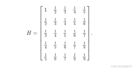
其数学性质非常"良好",但数值性质极其糟糕:
-
条件数随维度指数级增长
-
极小的输入扰动会导致解出现数量级放大的误差
在这种情况下:
-
无主元高斯消元 往往直接失败
-
列主元策略 能显著改善稳定性
-
迭代法(如共轭梯度) 在正定条件下反而更可靠
这说明:稳定性往往由"算法路径"决定,而非问题本身。
3. 高维优化中的误差放大效应
在数值优化中,稳定性问题往往以更加隐蔽的形式出现。
以高维梯度下降为例:
-
梯度计算本身包含舍入误差
-
学习率选择不当会放大这些误差
-
多次迭代后,误差呈指数级累积
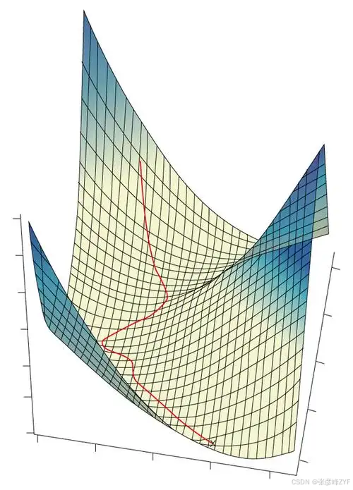
在一些病态目标函数(如狭长谷形的 Rosenbrock 函数)中:
-
梯度方向与最优下降方向严重偏离
-
数值误差会直接影响收敛路径
-
算法表面上"在下降",但实际效率极低
这也是为什么在工程实践中:
-
二阶或拟牛顿方法(BFGS / L-BFGS)
-
往往比一阶方法表现得更加"稳定且可靠"
4. 长迭代链路中的误差累积
在以下场景中,数值稳定性问题尤为突出:
-
大规模线性系统的迭代求解
-
时间步长很小的数值微分方程
-
深度学习中的长反向传播链路
其共同特征是:一次计算的微小误差,会在多次迭代中被反复放大。
如果算法本身不具备良好的数值稳定性,那么:
-
单步误差可能微不足道
-
多步误差却足以摧毁整个计算结果
5. 工程视角下的稳定性结论
从工程实践角度来看,可以得出几个非常现实的结论:
-
稳定性优先级高于理论最优复杂度
-
引入主元、正则化或缩放,往往比"换算法"更重要
-
对数值稳定性的忽视,通常不会立刻失败,而是"悄然失真"
这也是为什么在成熟数值计算库中:
-
很多"看似多余"的步骤(主元选择、重缩放、阈值判断)
-
实际上正是工程可靠性的核心保障
(三)时间与空间复杂度
复杂度不仅是 Big-O:
-
常数因子
-
内存访问模式
-
是否适合并行 / 向量化
在 JVM / CPU / Cache 体系下,这些因素往往比公式更重要。
(四)适用性(Applicability)
不存在"最优算法",只有"最适合场景的算法":
-
函数是否光滑?
-
问题规模是否巨大?
-
是否允许近似?
-
是否追求实时性?
二、整体框架设计
整个评估系统采用 "算法实现 + 评估分析" 的分层设计。
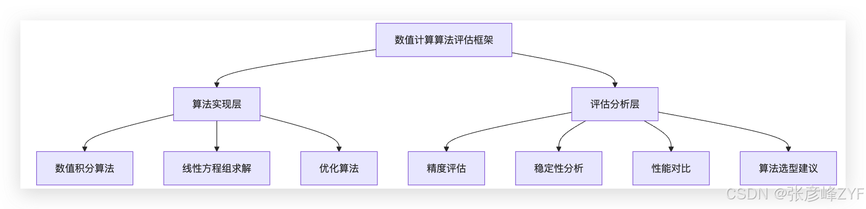
这种结构的核心优势在于:
-
算法与测试逻辑彻底解耦
-
易于横向扩展
-
支持系统性对比,而非"单点实验"
三、数值积分算法模块:精度与效率的平衡艺术
(一)数值积分的数学本质
目标是计算:

当解析积分不可得时,只能通过:离散采样 + 加权求和
(二)算法全景对比
| 方法 | 精度阶 | 特点 |
|---|---|---|
| 矩形法 | O(h) | 极简,误差大 |
| 梯形法 | O(h²) | 稳定、通用 |
| Simpson 法 | O(h⁴) | 工程常用 |
| 高斯积分 | 极高 | 光滑函数最优 |
| 自适应积分 | 自适应 | 鲁棒性强 |
| 蒙特卡洛 | O(1/√n) | 高维优势 |
(三)收敛性对比示意
在数值积分问题中,收敛性描述的是:当区间划分数逐渐增大(步长逐渐减小)时,数值结果逼近真实积分值的速度。
虽然不同算法的收敛阶可以通过严格的误差分析给出,但在工程实践中,更直观的理解方式是观察其误差随计算量增加的衰减趋势。
从定性角度来看,各类算法具有如下典型特征:
-
矩形法
随着区间数增加,误差呈线性下降趋势。即便计算量显著增加,精度提升依然有限,通常只适合教学或极低精度需求场景。
-
梯形法
误差下降速度明显快于矩形法,属于"性价比较高"的基础算法。在函数较为光滑时,随着区间细分,结果稳定逼近真实值。
-
Simpson 法则
对光滑函数表现出明显的高阶收敛特性。相较梯形法,在相同区间划分数下,其误差通常可降低一个甚至多个数量级,是工程中最常用的一维数值积分方法之一。
-
高斯积分
当被积函数足够光滑时,收敛速度极快,甚至在极少采样点的情况下即可获得高精度结果。但其优势高度依赖于函数的可平滑性。
-
自适应积分方法
不追求统一的全局收敛阶,而是通过局部误差控制,在函数变化剧烈的区域自动细分区间,在平缓区域减少计算量,从整体上实现更稳定、更高效的收敛行为。
总体而言,可以得到一个工程层面的结论:低阶方法依赖"更多计算量"换取精度,高阶与自适应方法则依赖"更合理的误差控制"实现快速收敛。
这也是在实际工程中,数值积分算法往往并非单纯依据理论复杂度选择,而是综合考虑函数特性、精度要求和计算成本后进行权衡。
(四)工程选型建议
-
通用一维积分:Simpson 法
-
高精度离线计算:高斯积分
-
函数变化剧烈:自适应 Simpson
-
高维积分:蒙特卡洛
四、线性方程组求解:稳定性优先于速度
(一)问题形式

这是所有数值计算中出现频率最高的问题。
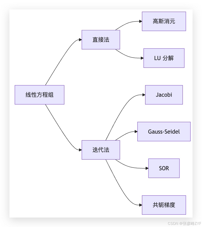
(二)方法分类
(三)病态矩阵:Hilbert 矩阵
Hilbert 矩阵是经典"反例":
-
条件数随维度指数增长
-
无主元消元法几乎必然失败
实验结论:
-
列主元显著提升稳定性
-
共轭梯度在正定条件下更可靠
(四)工程结论
-
小规模稠密矩阵 → LU
-
对称正定 → 共轭梯度
-
稀疏大规模 → 迭代法
五、优化算法模块:从数学收敛到工程效率
(一)一般形式

(二)方法对比
| 方法 | 收敛特性 | 工程评价 |
|---|---|---|
| 梯度下降 | 线性 | 慢但简单 |
| Adam | 稳定 | ML 首选 |
| 牛顿法 | 二次 | 代价高 |
| BFGS | 超线性 | 工程事实标准 |
| L-BFGS | 超线性 | 大规模首选 |
(三)统一评估框架的工程价值
该框架的核心价值在于:
-
统一评估标准
-
可重复实验设计
-
面向选型而非展示
非常适合作为:
-
教学平台
-
算法验证工具
-
工程基础库
六、简单验证说明
(一)项目结构概览
bash
numericalcomputation/
├── algorithms/          # 核心算法实现
│   ├── NumericalIntegration.java      # 数值积分(10种)
│   ├── LinearEquationSolvers.java     # 线性方程组求解(7种)
│   └── OptimizationAlgorithms.java    # 优化算法(6种)
├── evaluation/          # 统一评估与对比分析
│   ├── IntegrationPrecisionComparison.java
│   ├── LinearSolverEvaluation.java
│   └── OptimizationConvergenceAnalysis.java
└── performance/         # 性能测试
项目整体采用"算法实现 + 评估验证"的分层结构,便于算法对比、精度分析和后续扩展。
(二)核心模块快速说明
1. 数值积分模块
1.1 算法实现 NumericalIntegration
java
package org.zyf.javabasic.algorithm.numericalcomputation.algorithms;

import java.util.function.Function;

/**
 * @program: zyfboot-javabasic
 * @description: 数值积分算法实现
 * 包含矩形法则、梯形法则、辛普森法则和高斯积分等多种数值积分方法
 * @author: zhangyanfeng
 * @create: 2026-01-31 15:27
 **/
public class NumericalIntegration {

    /**
     * 矩形法则(左端点)
     * 时间复杂度: O(n)
     * 精度: O(h),其中h = (b-a)/n
     */
    public static double rectangleRule(Function<Double, Double> f, double a, double b, int n) {
        double h = (b - a) / n;
        double sum = 0.0;

        for (int i = 0; i < n; i++) {
            double x = a + i * h;
            sum += f.apply(x);
        }

        return h * sum;
    }

    /**
     * 矩形法则(中点)
     * 时间复杂度: O(n)
     * 精度: O(h²),其中h = (b-a)/n
     */
    public static double midpointRule(Function<Double, Double> f, double a, double b, int n) {
        double h = (b - a) / n;
        double sum = 0.0;

        for (int i = 0; i < n; i++) {
            double x = a + (i + 0.5) * h;
            sum += f.apply(x);
        }

        return h * sum;
    }

    /**
     * 梯形法则
     * 时间复杂度: O(n)
     * 精度: O(h²),其中h = (b-a)/n
     */
    public static double trapezoidalRule(Function<Double, Double> f, double a, double b, int n) {
        double h = (b - a) / n;
        double sum = 0.5 * (f.apply(a) + f.apply(b));

        for (int i = 1; i < n; i++) {
            double x = a + i * h;
            sum += f.apply(x);
        }

        return h * sum;
    }

    /**
     * 辛普森法则(1/3法则)
     * 时间复杂度: O(n)
     * 精度: O(h⁴),其中h = (b-a)/n
     */
    public static double simpsonsRule(Function<Double, Double> f, double a, double b, int n) {
        if (n % 2 != 0) {
            throw new IllegalArgumentException("Simpson's rule requires even number of intervals");
        }

        double h = (b - a) / n;
        double sum = f.apply(a) + f.apply(b);

        // 奇数点
        for (int i = 1; i < n; i += 2) {
            double x = a + i * h;
            sum += 4 * f.apply(x);
        }

        // 偶数点
        for (int i = 2; i < n; i += 2) {
            double x = a + i * h;
            sum += 2 * f.apply(x);
        }

        return h * sum / 3.0;
    }

    /**
     * 辛普森法则(3/8法则)
     * 时间复杂度: O(n)
     * 精度: O(h⁴),其中h = (b-a)/n
     */
    public static double simpsons38Rule(Function<Double, Double> f, double a, double b, int n) {
        if (n % 3 != 0) {
            throw new IllegalArgumentException("Simpson's 3/8 rule requires number of intervals divisible by 3");
        }

        double h = (b - a) / n;
        double sum = f.apply(a) + f.apply(b);

        for (int i = 1; i < n; i++) {
            double x = a + i * h;
            if (i % 3 == 0) {
                sum += 2 * f.apply(x);
            } else {
                sum += 3 * f.apply(x);
            }
        }

        return 3 * h * sum / 8.0;
    }

    /**
     * 2点高斯积分
     * 时间复杂度: O(1)
     * 精度: 对于3次多项式精确
     */
    public static double gaussianQuadrature2Point(Function<Double, Double> f, double a, double b) {
        // 变换到标准区间[-1, 1]
        double center = (a + b) / 2.0;
        double halfWidth = (b - a) / 2.0;

        // 2点高斯积分的节点和权重
        double[] nodes = {-0.5773502691896257, 0.5773502691896257};
        double[] weights = {1.0, 1.0};

        double sum = 0.0;
        for (int i = 0; i < nodes.length; i++) {
            double x = center + halfWidth * nodes[i];
            sum += weights[i] * f.apply(x);
        }

        return halfWidth * sum;
    }

    /**
     * 3点高斯积分
     * 时间复杂度: O(1)
     * 精度: 对于5次多项式精确
     */
    public static double gaussianQuadrature3Point(Function<Double, Double> f, double a, double b) {
        // 变换到标准区间[-1, 1]
        double center = (a + b) / 2.0;
        double halfWidth = (b - a) / 2.0;

        // 3点高斯积分的节点和权重
        double[] nodes = {-0.7745966692414834, 0.0, 0.7745966692414834};
        double[] weights = {0.5555555555555556, 0.8888888888888888, 0.5555555555555556};

        double sum = 0.0;
        for (int i = 0; i < nodes.length; i++) {
            double x = center + halfWidth * nodes[i];
            sum += weights[i] * f.apply(x);
        }

        return halfWidth * sum;
    }

    /**
     * 4点高斯积分
     * 时间复杂度: O(1)
     * 精度: 对于7次多项式精确
     */
    public static double gaussianQuadrature4Point(Function<Double, Double> f, double a, double b) {
        // 变换到标准区间[-1, 1]
        double center = (a + b) / 2.0;
        double halfWidth = (b - a) / 2.0;

        // 4点高斯积分的节点和权重
        double[] nodes = {-0.8611363115940526, -0.3399810435848563, 0.3399810435848563, 0.8611363115940526};
        double[] weights = {0.3478548451374538, 0.6521451548625461, 0.6521451548625461, 0.3478548451374538};

        double sum = 0.0;
        for (int i = 0; i < nodes.length; i++) {
            double x = center + halfWidth * nodes[i];
            sum += weights[i] * f.apply(x);
        }

        return halfWidth * sum;
    }

    /**
     * 自适应积分(递归实现)
     * 基于辛普森法则的自适应算法
     * 时间复杂度: O(log(ε)),其中ε是误差容忍度
     */
    public static double adaptiveIntegration(Function<Double, Double> f, double a, double b, double tolerance) {
        return adaptiveSimpsonsRecursive(f, a, b, tolerance, simpsonsRule(f, a, b, 2), 0);
    }

    private static double adaptiveSimpsonsRecursive(Function<Double, Double> f, double a, double b,
                                                    double tolerance, double wholeArea, int depth) {
        if (depth > 50) { // 防止无限递归
            return wholeArea;
        }

        double c = (a + b) / 2.0;
        double leftArea = simpsonsRule(f, a, c, 2);
        double rightArea = simpsonsRule(f, c, b, 2);
        double totalArea = leftArea + rightArea;

        double error = Math.abs(totalArea - wholeArea) / 15.0; // 误差估计

        if (error < tolerance) {
            return totalArea + error; // 理查德森外推法修正
        } else {
            return adaptiveSimpsonsRecursive(f, a, c, tolerance/2.0, leftArea, depth+1) +
                    adaptiveSimpsonsRecursive(f, c, b, tolerance/2.0, rightArea, depth+1);
        }
    }

    /**
     * 蒙特卡洛积分
     * 时间复杂度: O(n)
     * 精度: O(1/√n),收敛速度与维度无关
     */
    public static double monteCarloIntegration(Function<Double, Double> f, double a, double b, int n) {
        double sum = 0.0;
        java.util.Random random = new java.util.Random();

        for (int i = 0; i < n; i++) {
            double x = a + (b - a) * random.nextDouble();
            sum += f.apply(x);
        }

        return (b - a) * sum / n;
    }
}已实现常见一维数值积分方法,覆盖低阶 → 高阶 → 自适应 → 随机方法:
-
基础方法
-
矩形法(左端点 / 中点):
O(h)/O(h²) -
梯形法:
O(h²),稳定可靠
-
-
高阶方法
-
辛普森法(1/3、3/8):
O(h⁴) -
高斯积分(2--4点):高精度、低计算量
-
-
特殊方法
-
自适应辛普森:自动控制误差
-
蒙特卡洛积分:适合多维问题,
O(1/√n)收敛
-
1.2 精度评估(IntegrationPrecisionComparison.java)
-
测试函数:多项式、三角、指数、对数、振荡函数等
-
评估维度:
-
收敛速度(区间数 vs 误差)
-
计算效率
-
数值稳定性
-
-
输出结果:不同函数类型下的算法推荐结论(见后续统一测试)
具体代码验证:
java
package org.zyf.javabasic.algorithm.numericalcomputation.evaluation;

import org.zyf.javabasic.algorithm.numericalcomputation.algorithms.NumericalIntegration;

import java.util.*;
import java.util.function.Function;

/**
 * @program: zyfboot-javabasic
 * @description: 数值积分方法精度对比分析
 * 系统性评估不同数值积分方法在各种测试函数上的精度表现
 * @author: zhangyanfeng
 * @create: 2026-01-31 15:27
 **/
public class IntegrationPrecisionComparison {

    /**
     * 积分方法评估结果
     */
    public static class IntegrationResult {
        public String methodName;
        public double result;
        public double error;
        public double relativeError;
        public long computationTime; // 纳秒
        public int evaluations; // 函数评估次数

        public IntegrationResult(String methodName, double result, double exactValue,
                                 long computationTime, int evaluations) {
            this.methodName = methodName;
            this.result = result;
            this.error = Math.abs(result - exactValue);
            this.relativeError = exactValue != 0 ? this.error / Math.abs(exactValue) : Double.MAX_VALUE;
            this.computationTime = computationTime;
            this.evaluations = evaluations;
        }

        @Override
        public String toString() {
            return String.format("%s: 结果=%.8f, 绝对误差=%.2e, 相对误差=%.2e, 时间=%dns, 评估次数=%d",
                    methodName, result, error, relativeError, computationTime, evaluations);
        }
    }

    /**
     * 测试函数接口
     */
    public interface TestFunction {
        Function<Double, Double> getFunction();
        double getExactIntegral(double a, double b);
        String getName();
        String getDescription();
    }

    /**
     * 预定义测试函数
     */
    public static class TestFunctions {
        // f(x) = x^2, ∫[0,1] x^2 dx = 1/3
        public static final TestFunction POLYNOMIAL = new TestFunction() {
            @Override
            public Function<Double, Double> getFunction() {
                return x -> x * x;
            }

            @Override
            public double getExactIntegral(double a, double b) {
                return (b * b * b - a * a * a) / 3.0;
            }

            @Override
            public String getName() {
                return "多项式函数";
            }

            @Override
            public String getDescription() {
                return "f(x) = x²";
            }
        };

        // f(x) = sin(x), ∫[0,π] sin(x) dx = 2
        public static final TestFunction TRIGONOMETRIC = new TestFunction() {
            @Override
            public Function<Double, Double> getFunction() {
                return Math::sin;
            }

            @Override
            public double getExactIntegral(double a, double b) {
                return -Math.cos(b) + Math.cos(a);
            }

            @Override
            public String getName() {
                return "三角函数";
            }

            @Override
            public String getDescription() {
                return "f(x) = sin(x)";
            }
        };

        // f(x) = e^x, ∫[0,1] e^x dx = e - 1
        public static final TestFunction EXPONENTIAL = new TestFunction() {
            @Override
            public Function<Double, Double> getFunction() {
                return Math::exp;
            }

            @Override
            public double getExactIntegral(double a, double b) {
                return Math.exp(b) - Math.exp(a);
            }

            @Override
            public String getName() {
                return "指数函数";
            }

            @Override
            public String getDescription() {
                return "f(x) = e^x";
            }
        };

        // f(x) = 1/x, ∫[1,e] 1/x dx = 1
        public static final TestFunction LOGARITHMIC = new TestFunction() {
            @Override
            public Function<Double, Double> getFunction() {
                return x -> 1.0 / x;
            }

            @Override
            public double getExactIntegral(double a, double b) {
                return Math.log(b) - Math.log(a);
            }

            @Override
            public String getName() {
                return "对数函数";
            }

            @Override
            public String getDescription() {
                return "f(x) = 1/x";
            }
        };

        // f(x) = sqrt(1 - x^2), ∫[-1,1] sqrt(1-x²) dx = π/2 (半圆)
        public static final TestFunction SEMICIRCLE = new TestFunction() {
            @Override
            public Function<Double, Double> getFunction() {
                return x -> Math.sqrt(1.0 - x * x);
            }

            @Override
            public double getExactIntegral(double a, double b) {
                // 这是半圆函数,在[-1,1]上积分为π/2
                if (a == -1.0 && b == 1.0) {
                    return Math.PI / 2.0;
                }
                // 对于其他区间,使用数值近似
                return Math.PI / 2.0 * (b - a) / 2.0;
            }

            @Override
            public String getName() {
                return "半圆函数";
            }

            @Override
            public String getDescription() {
                return "f(x) = √(1-x²)";
            }
        };

        // f(x) = x * sin(x), ∫[0,π] x*sin(x) dx = π
        public static final TestFunction OSCILLATORY = new TestFunction() {
            @Override
            public Function<Double, Double> getFunction() {
                return x -> x * Math.sin(x);
            }

            @Override
            public double getExactIntegral(double a, double b) {
                // ∫ x*sin(x) dx = sin(x) - x*cos(x)
                return (Math.sin(b) - b * Math.cos(b)) - (Math.sin(a) - a * Math.cos(a));
            }

            @Override
            public String getName() {
                return "振荡函数";
            }

            @Override
            public String getDescription() {
                return "f(x) = x·sin(x)";
            }
        };
    }

    /**
     * 执行精度比较测试
     */
    public static List<IntegrationResult> compareIntegrationMethods(TestFunction testFunction,
                                                                    double a, double b, int n) {
        List<IntegrationResult> results = new ArrayList<>();
        double exactValue = testFunction.getExactIntegral(a, b);
        Function<Double, Double> f = testFunction.getFunction();

        // 矩形法则(左端点)
        long start = System.nanoTime();
        double result1 = NumericalIntegration.rectangleRule(f, a, b, n);
        long end = System.nanoTime();
        results.add(new IntegrationResult("矩形法则(左端点)", result1, exactValue, end - start, n));

        // 矩形法则(中点)
        start = System.nanoTime();
        double result2 = NumericalIntegration.midpointRule(f, a, b, n);
        end = System.nanoTime();
        results.add(new IntegrationResult("矩形法则(中点)", result2, exactValue, end - start, n));

        // 梯形法则
        start = System.nanoTime();
        double result3 = NumericalIntegration.trapezoidalRule(f, a, b, n);
        end = System.nanoTime();
        results.add(new IntegrationResult("梯形法则", result3, exactValue, end - start, n + 1));

        // 辛普森法则(确保n为偶数)
        int evenN = (n % 2 == 0) ? n : n - 1;
        if (evenN >= 2) {
            start = System.nanoTime();
            double result4 = NumericalIntegration.simpsonsRule(f, a, b, evenN);
            end = System.nanoTime();
            results.add(new IntegrationResult("辛普森法则(1/3)", result4, exactValue, end - start, evenN + 1));
        }

        // 辛普森3/8法则(确保n能被3整除)
        int divisibleBy3N = (n / 3) * 3;
        if (divisibleBy3N >= 3) {
            start = System.nanoTime();
            double result5 = NumericalIntegration.simpsons38Rule(f, a, b, divisibleBy3N);
            end = System.nanoTime();
            results.add(new IntegrationResult("辛普森法则(3/8)", result5, exactValue, end - start, divisibleBy3N + 1));
        }

        // 高斯积分
        start = System.nanoTime();
        double result6 = NumericalIntegration.gaussianQuadrature2Point(f, a, b);
        end = System.nanoTime();
        results.add(new IntegrationResult("高斯积分(2点)", result6, exactValue, end - start, 2));

        start = System.nanoTime();
        double result7 = NumericalIntegration.gaussianQuadrature3Point(f, a, b);
        end = System.nanoTime();
        results.add(new IntegrationResult("高斯积分(3点)", result7, exactValue, end - start, 3));

        start = System.nanoTime();
        double result8 = NumericalIntegration.gaussianQuadrature4Point(f, a, b);
        end = System.nanoTime();
        results.add(new IntegrationResult("高斯积分(4点)", result8, exactValue, end - start, 4));

        // 自适应积分
        start = System.nanoTime();
        double result9 = NumericalIntegration.adaptiveIntegration(f, a, b, 1e-10);
        end = System.nanoTime();
        results.add(new IntegrationResult("自适应积分", result9, exactValue, end - start, -1));

        // 蒙特卡洛积分
        start = System.nanoTime();
        double result10 = NumericalIntegration.monteCarloIntegration(f, a, b, n * 10);
        end = System.nanoTime();
        results.add(new IntegrationResult("蒙特卡洛积分", result10, exactValue, end - start, n * 10));

        return results;
    }

    /**
     * 生成精度收敛分析报告
     */
    public static void convergenceAnalysis(TestFunction testFunction, double a, double b) {
        System.out.println("=== 收敛性分析: " + testFunction.getName() + " ===");
        System.out.println("函数: " + testFunction.getDescription());
        System.out.println("积分区间: [" + a + ", " + b + "]");
        System.out.println("精确值: " + testFunction.getExactIntegral(a, b));
        System.out.println();

        int[] intervals = {10, 50, 100, 500, 1000};

        for (int n : intervals) {
            System.out.println("--- 区间数: " + n + " ---");
            List<IntegrationResult> results = compareIntegrationMethods(testFunction, a, b, n);

            // 按精度排序
            results.sort(Comparator.comparingDouble(r -> r.error));

            for (IntegrationResult result : results) {
                System.out.println(result);
            }
            System.out.println();
        }
    }

    /**
     * 综合评估不同积分方法
     */
    public static void comprehensiveEvaluation() {
        System.out.println("=== 数值积分方法综合精度对比分析 ===");
        System.out.println("评估维度:精度、效率、稳定性");
        System.out.println();

        TestFunction[] functions = {
                TestFunctions.POLYNOMIAL,
                TestFunctions.TRIGONOMETRIC,
                TestFunctions.EXPONENTIAL,
                TestFunctions.LOGARITHMIC,
                TestFunctions.SEMICIRCLE,
                TestFunctions.OSCILLATORY
        };

        double[][] intervals = {
                {0, 1},      // 多项式
                {0, Math.PI}, // 三角函数
                {0, 1},      // 指数函数
                {1, Math.E}, // 对数函数
                {-1, 1},     // 半圆函数
                {0, Math.PI} // 振荡函数
        };

        Map<String, List<Double>> methodErrors = new HashMap<>();
        Map<String, List<Long>> methodTimes = new HashMap<>();

        for (int i = 0; i < functions.length; i++) {
            TestFunction func = functions[i];
            double a = intervals[i][0];
            double b = intervals[i][1];

            System.out.println("=== " + func.getName() + " ===");
            List<IntegrationResult> results = compareIntegrationMethods(func, a, b, 100);

            for (IntegrationResult result : results) {
                methodErrors.computeIfAbsent(result.methodName, k -> new ArrayList<>())
                        .add(result.relativeError);
                methodTimes.computeIfAbsent(result.methodName, k -> new ArrayList<>())
                        .add(result.computationTime);
                System.out.println(result);
            }
            System.out.println();
        }

        // 生成综合评估报告
        generateSummaryReport(methodErrors, methodTimes);
    }

    /**
     * 生成综合评估报告
     */
    private static void generateSummaryReport(Map<String, List<Double>> methodErrors,
                                              Map<String, List<Long>> methodTimes) {
        System.out.println("=== 综合评估报告 ===");

        List<String> methods = new ArrayList<>(methodErrors.keySet());
        methods.sort(String::compareTo);

        System.out.printf("%-20s %15s %15s %15s %15s%n",
                "方法", "平均相对误差", "最大相对误差", "平均时间(ns)", "稳定性评分");
        StringBuilder separator = new StringBuilder();
        for (int i = 0; i < 85; i++) {
            separator.append("-");
        }
        System.out.println(separator.toString());

        for (String method : methods) {
            List<Double> errors = methodErrors.get(method);
            List<Long> times = methodTimes.get(method);

            double avgError = errors.stream().mapToDouble(Double::doubleValue).average().orElse(0);
            double maxError = errors.stream().mapToDouble(Double::doubleValue).max().orElse(0);
            double avgTime = times.stream().mapToLong(Long::longValue).average().orElse(0);

            // 稳定性评分:基于误差的变异系数
            double errorStdDev = calculateStandardDeviation(errors);
            double stabilityScore = avgError > 0 ? Math.max(0, 10 - (errorStdDev / avgError) * 10) : 10;

            System.out.printf("%-20s %15.2e %15.2e %15.0f %15.1f%n",
                    method, avgError, maxError, avgTime, stabilityScore);
        }

        System.out.println();
        generateRecommendations(methodErrors, methodTimes);
    }

    /**
     * 计算标准差
     */
    private static double calculateStandardDeviation(List<Double> values) {
        double mean = values.stream().mapToDouble(Double::doubleValue).average().orElse(0);
        double variance = values.stream()
                .mapToDouble(x -> (x - mean) * (x - mean))
                .average().orElse(0);
        return Math.sqrt(variance);
    }

    /**
     * 生成算法推荐
     */
    private static void generateRecommendations(Map<String, List<Double>> methodErrors,
                                                Map<String, List<Long>> methodTimes) {
        System.out.println("=== 算法选择建议 ===");
        System.out.println("1. 高精度需求: 推荐自适应积分或高阶高斯积分");
        System.out.println("2. 快速计算: 推荐高斯积分(2-3点)或辛普森法则");
        System.out.println("3. 光滑函数: 推荐高斯积分或辛普森法则");
        System.out.println("4. 振荡函数: 推荐自适应积分");
        System.out.println("5. 多维积分: 推荐蒙特卡洛方法");
        System.out.println("6. 通用选择: 推荐辛普森法则或梯形法则");
        System.out.println();
    }

    /**
     * 示例主函数
     */
    public static void main(String[] args) {
        System.out.println("数值积分方法精度对比分析演示");
        StringBuilder header = new StringBuilder();
        for (int i = 0; i < 50; i++) {
            header.append("=");
        }
        System.out.println(header.toString());

        // 单个函数收敛性分析
        convergenceAnalysis(TestFunctions.POLYNOMIAL, 0, 1);

        // 综合评估
        comprehensiveEvaluation();
    }
}
执行展示:
数值积分方法精度对比分析演示
==================================================
=== 收敛性分析: 多项式函数 ===
函数: f(x) = x²
积分区间: 0.0, 1.0
精确值: 0.3333333333333333
--- 区间数: 10 ---
辛普森法则(3/8): 结果=0.33333333, 绝对误差=5.55e-17, 相对误差=1.67e-16, 时间=12041ns, 评估次数=10
高斯积分(2点): 结果=0.33333333, 绝对误差=5.55e-17, 相对误差=1.67e-16, 时间=3375ns, 评估次数=2
高斯积分(3点): 结果=0.33333333, 绝对误差=5.55e-17, 相对误差=1.67e-16, 时间=4000ns, 评估次数=3
高斯积分(4点): 结果=0.33333333, 绝对误差=5.55e-17, 相对误差=1.67e-16, 时间=5083ns, 评估次数=4
自适应积分: 结果=0.33333333, 绝对误差=5.55e-17, 相对误差=1.67e-16, 时间=13833ns, 评估次数=-1
辛普森法则(1/3): 结果=0.33333333, 绝对误差=1.67e-16, 相对误差=5.00e-16, 时间=13042ns, 评估次数=11
矩形法则(中点): 结果=0.33250000, 绝对误差=8.33e-04, 相对误差=2.50e-03, 时间=12916ns, 评估次数=10
梯形法则: 结果=0.33500000, 绝对误差=1.67e-03, 相对误差=5.00e-03, 时间=13500ns, 评估次数=11
蒙特卡洛积分: 结果=0.35656091, 绝对误差=2.32e-02, 相对误差=6.97e-02, 时间=343625ns, 评估次数=100
矩形法则(左端点): 结果=0.28500000, 绝对误差=4.83e-02, 相对误差=1.45e-01, 时间=478375ns, 评估次数=10
--- 区间数: 50 ---
辛普森法则(1/3): 结果=0.33333333, 绝对误差=0.00e+00, 相对误差=0.00e+00, 时间=11541ns, 评估次数=51
辛普森法则(3/8): 结果=0.33333333, 绝对误差=0.00e+00, 相对误差=0.00e+00, 时间=16500ns, 评估次数=49
高斯积分(2点): 结果=0.33333333, 绝对误差=5.55e-17, 相对误差=1.67e-16, 时间=1833ns, 评估次数=2
高斯积分(3点): 结果=0.33333333, 绝对误差=5.55e-17, 相对误差=1.67e-16, 时间=1458ns, 评估次数=3
高斯积分(4点): 结果=0.33333333, 绝对误差=5.55e-17, 相对误差=1.67e-16, 时间=1584ns, 评估次数=4
自适应积分: 结果=0.33333333, 绝对误差=5.55e-17, 相对误差=1.67e-16, 时间=3541ns, 评估次数=-1
矩形法则(中点): 结果=0.33330000, 绝对误差=3.33e-05, 相对误差=1.00e-04, 时间=39750ns, 评估次数=50
梯形法则: 结果=0.33340000, 绝对误差=6.67e-05, 相对误差=2.00e-04, 时间=16875ns, 评估次数=51
蒙特卡洛积分: 结果=0.32543127, 绝对误差=7.90e-03, 相对误差=2.37e-02, 时间=331500ns, 评估次数=500
矩形法则(左端点): 结果=0.32340000, 绝对误差=9.93e-03, 相对误差=2.98e-02, 时间=43209ns, 评估次数=50
--- 区间数: 100 ---
辛普森法则(3/8): 结果=0.33333333, 绝对误差=5.55e-17, 相对误差=1.67e-16, 时间=7833ns, 评估次数=100
高斯积分(2点): 结果=0.33333333, 绝对误差=5.55e-17, 相对误差=1.67e-16, 时间=1083ns, 评估次数=2
高斯积分(3点): 结果=0.33333333, 绝对误差=5.55e-17, 相对误差=1.67e-16, 时间=833ns, 评估次数=3
高斯积分(4点): 结果=0.33333333, 绝对误差=5.55e-17, 相对误差=1.67e-16, 时间=667ns, 评估次数=4
自适应积分: 结果=0.33333333, 绝对误差=5.55e-17, 相对误差=1.67e-16, 时间=2625ns, 评估次数=-1
辛普森法则(1/3): 结果=0.33333333, 绝对误差=1.11e-16, 相对误差=3.33e-16, 时间=5375ns, 评估次数=101
矩形法则(中点): 结果=0.33332500, 绝对误差=8.33e-06, 相对误差=2.50e-05, 时间=25583ns, 评估次数=100
梯形法则: 结果=0.33335000, 绝对误差=1.67e-05, 相对误差=5.00e-05, 时间=13958ns, 评估次数=101
矩形法则(左端点): 结果=0.32835000, 绝对误差=4.98e-03, 相对误差=1.49e-02, 时间=27916ns, 评估次数=100
蒙特卡洛积分: 结果=0.35576427, 绝对误差=2.24e-02, 相对误差=6.73e-02, 时间=90583ns, 评估次数=1000
--- 区间数: 500 ---
辛普森法则(1/3): 结果=0.33333333, 绝对误差=0.00e+00, 相对误差=0.00e+00, 时间=28500ns, 评估次数=501
高斯积分(2点): 结果=0.33333333, 绝对误差=5.55e-17, 相对误差=1.67e-16, 时间=1250ns, 评估次数=2
高斯积分(3点): 结果=0.33333333, 绝对误差=5.55e-17, 相对误差=1.67e-16, 时间=625ns, 评估次数=3
高斯积分(4点): 结果=0.33333333, 绝对误差=5.55e-17, 相对误差=1.67e-16, 时间=583ns, 评估次数=4
自适应积分: 结果=0.33333333, 绝对误差=5.55e-17, 相对误差=1.67e-16, 时间=1417ns, 评估次数=-1
辛普森法则(3/8): 结果=0.33333333, 绝对误差=2.22e-16, 相对误差=6.66e-16, 时间=29875ns, 评估次数=499
矩形法则(中点): 结果=0.33333300, 绝对误差=3.33e-07, 相对误差=1.00e-06, 时间=30167ns, 评估次数=500
梯形法则: 结果=0.33333400, 绝对误差=6.67e-07, 相对误差=2.00e-06, 时间=27292ns, 评估次数=501
蒙特卡洛积分: 结果=0.33391469, 绝对误差=5.81e-04, 相对误差=1.74e-03, 时间=398459ns, 评估次数=5000
矩形法则(左端点): 结果=0.33233400, 绝对误差=9.99e-04, 相对误差=3.00e-03, 时间=35709ns, 评估次数=500
--- 区间数: 1000 ---
辛普森法则(1/3): 结果=0.33333333, 绝对误差=0.00e+00, 相对误差=0.00e+00, 时间=92666ns, 评估次数=1001
辛普森法则(3/8): 结果=0.33333333, 绝对误差=0.00e+00, 相对误差=0.00e+00, 时间=51166ns, 评估次数=1000
高斯积分(2点): 结果=0.33333333, 绝对误差=5.55e-17, 相对误差=1.67e-16, 时间=958ns, 评估次数=2
高斯积分(3点): 结果=0.33333333, 绝对误差=5.55e-17, 相对误差=1.67e-16, 时间=625ns, 评估次数=3
高斯积分(4点): 结果=0.33333333, 绝对误差=5.55e-17, 相对误差=1.67e-16, 时间=625ns, 评估次数=4
自适应积分: 结果=0.33333333, 绝对误差=5.55e-17, 相对误差=1.67e-16, 时间=1333ns, 评估次数=-1
矩形法则(中点): 结果=0.33333325, 绝对误差=8.33e-08, 相对误差=2.50e-07, 时间=46250ns, 评估次数=1000
梯形法则: 结果=0.33333350, 绝对误差=1.67e-07, 相对误差=5.00e-07, 时间=48167ns, 评估次数=1001
矩形法则(左端点): 结果=0.33283350, 绝对误差=5.00e-04, 相对误差=1.50e-03, 时间=47250ns, 评估次数=1000
蒙特卡洛积分: 结果=0.32957485, 绝对误差=3.76e-03, 相对误差=1.13e-02, 时间=561167ns, 评估次数=10000
=== 数值积分方法综合精度对比分析 ===
评估维度:精度、效率、稳定性
=== 多项式函数 ===
矩形法则(左端点): 结果=0.32835000, 绝对误差=4.98e-03, 相对误差=1.49e-02, 时间=5166ns, 评估次数=100
矩形法则(中点): 结果=0.33332500, 绝对误差=8.33e-06, 相对误差=2.50e-05, 时间=6750ns, 评估次数=100
梯形法则: 结果=0.33335000, 绝对误差=1.67e-05, 相对误差=5.00e-05, 时间=4667ns, 评估次数=101
辛普森法则(1/3): 结果=0.33333333, 绝对误差=1.11e-16, 相对误差=3.33e-16, 时间=4833ns, 评估次数=101
辛普森法则(3/8): 结果=0.33333333, 绝对误差=5.55e-17, 相对误差=1.67e-16, 时间=5458ns, 评估次数=100
高斯积分(2点): 结果=0.33333333, 绝对误差=5.55e-17, 相对误差=1.67e-16, 时间=750ns, 评估次数=2
高斯积分(3点): 结果=0.33333333, 绝对误差=5.55e-17, 相对误差=1.67e-16, 时间=666ns, 评估次数=3
高斯积分(4点): 结果=0.33333333, 绝对误差=5.55e-17, 相对误差=1.67e-16, 时间=750ns, 评估次数=4
自适应积分: 结果=0.33333333, 绝对误差=5.55e-17, 相对误差=1.67e-16, 时间=2417ns, 评估次数=-1
蒙特卡洛积分: 结果=0.32323347, 绝对误差=1.01e-02, 相对误差=3.03e-02, 时间=58291ns, 评估次数=1000
=== 三角函数 ===
矩形法则(左端点): 结果=1.99983550, 绝对误差=1.64e-04, 相对误差=8.22e-05, 时间=21750ns, 评估次数=100
矩形法则(中点): 结果=2.00008225, 绝对误差=8.22e-05, 相对误差=4.11e-05, 时间=18334ns, 评估次数=100
梯形法则: 结果=1.99983550, 绝对误差=1.64e-04, 相对误差=8.22e-05, 时间=20917ns, 评估次数=101
辛普森法则(1/3): 结果=2.00000001, 绝对误差=1.08e-08, 相对误差=5.41e-09, 时间=17167ns, 评估次数=101
辛普森法则(3/8): 结果=2.00000003, 绝对误差=2.54e-08, 相对误差=1.27e-08, 时间=18709ns, 评估次数=100
高斯积分(2点): 结果=1.93581957, 绝对误差=6.42e-02, 相对误差=3.21e-02, 时间=1250ns, 评估次数=2
高斯积分(3点): 结果=2.00138891, 绝对误差=1.39e-03, 相对误差=6.94e-04, 时间=1167ns, 评估次数=3
高斯积分(4点): 结果=1.99998423, 绝对误差=1.58e-05, 相对误差=7.89e-06, 时间=1083ns, 评估次数=4
自适应积分: 结果=2.00000000, 绝对误差=4.57e-11, 相对误差=2.28e-11, 时间=278375ns, 评估次数=-1
蒙特卡洛积分: 结果=1.99458024, 绝对误差=5.42e-03, 相对误差=2.71e-03, 时间=129792ns, 评估次数=1000
=== 指数函数 ===
矩形法则(左端点): 结果=1.70970474, 绝对误差=8.58e-03, 相对误差=4.99e-03, 时间=20542ns, 评估次数=100
矩形法则(中点): 结果=1.71827467, 绝对误差=7.16e-06, 相对误差=4.17e-06, 时间=20333ns, 评估次数=100
梯形法则: 结果=1.71829615, 绝对误差=1.43e-05, 相对误差=8.33e-06, 时间=16541ns, 评估次数=101
辛普森法则(1/3): 结果=1.71828183, 绝对误差=9.55e-11, 相对误差=5.56e-11, 时间=32458ns, 评估次数=101
辛普森法则(3/8): 结果=1.71828183, 绝对误差=2.24e-10, 相对误差=1.30e-10, 时间=17250ns, 评估次数=100
高斯积分(2点): 结果=1.71789638, 绝对误差=3.85e-04, 相对误差=2.24e-04, 时间=1208ns, 评估次数=2
高斯积分(3点): 结果=1.71828100, 绝对误差=8.24e-07, 相对误差=4.80e-07, 时间=1000ns, 评估次数=3
高斯积分(4点): 结果=1.71828183, 绝对误差=9.33e-10, 相对误差=5.43e-10, 时间=1083ns, 评估次数=4
自适应积分: 结果=1.71828183, 绝对误差=7.11e-11, 相对误差=4.14e-11, 时间=70791ns, 评估次数=-1
蒙特卡洛积分: 结果=1.72913374, 绝对误差=1.09e-02, 相对误差=6.32e-03, 时间=172875ns, 评估次数=1000
=== 对数函数 ===
矩形法则(左端点): 结果=1.00545208, 绝对误差=5.45e-03, 相对误差=5.45e-03, 时间=31667ns, 评估次数=100
矩形法则(中点): 结果=0.99998936, 绝对误差=1.06e-05, 相对误差=1.06e-05, 时间=28875ns, 评估次数=100
梯形法则: 结果=1.00002127, 绝对误差=2.13e-05, 相对误差=2.13e-05, 时间=32708ns, 评估次数=101
辛普森法则(1/3): 结果=1.00000000, 绝对误差=2.85e-09, 相对误差=2.85e-09, 时间=48083ns, 评估次数=101
辛普森法则(3/8): 结果=1.00000001, 绝对误差=6.67e-09, 相对误差=6.67e-09, 时间=29042ns, 评估次数=100
高斯积分(2点): 结果=0.99506727, 绝对误差=4.93e-03, 相对误差=4.93e-03, 时间=1416ns, 评估次数=2
高斯积分(3点): 结果=0.99969382, 绝对误差=3.06e-04, 相对误差=3.06e-04, 时间=1292ns, 评估次数=3
高斯积分(4点): 结果=0.99998129, 绝对误差=1.87e-05, 相对误差=1.87e-05, 时间=1666ns, 评估次数=4
自适应积分: 结果=1.00000000, 绝对误差=7.45e-11, 相对误差=7.45e-11, 时间=145000ns, 评估次数=-1
蒙特卡洛积分: 结果=1.01032854, 绝对误差=1.03e-02, 相对误差=1.03e-02, 时间=64709ns, 评估次数=1000
=== 半圆函数 ===
矩形法则(左端点): 结果=1.56913426, 绝对误差=1.66e-03, 相对误差=1.06e-03, 时间=32209ns, 评估次数=100
矩形法则(中点): 结果=1.57128278, 绝对误差=4.86e-04, 相对误差=3.10e-04, 时间=30917ns, 评估次数=100
梯形法则: 结果=1.56913426, 绝对误差=1.66e-03, 相对误差=1.06e-03, 时间=28708ns, 评估次数=101
辛普森法则(1/3): 结果=1.57014629, 绝对误差=6.50e-04, 相对误差=4.14e-04, 时间=27625ns, 评估次数=101
辛普森法则(3/8): 结果=1.56999269, 绝对误差=8.04e-04, 相对误差=5.12e-04, 时间=27500ns, 评估次数=100
高斯积分(2点): 结果=1.63299316, 绝对误差=6.22e-02, 相对误差=3.96e-02, 时间=1292ns, 评估次数=2
高斯积分(3点): 结果=1.59161726, 绝对误差=2.08e-02, 相对误差=1.33e-02, 时间=1375ns, 评估次数=3
高斯积分(4点): 结果=1.58027753, 绝对误差=9.48e-03, 相对误差=6.04e-03, 时间=1583ns, 评估次数=4
自适应积分: 结果=1.57079633, 绝对误差=1.15e-14, 相对误差=7.35e-15, 时间=762500ns, 评估次数=-1
蒙特卡洛积分: 结果=1.56746647, 绝对误差=3.33e-03, 相对误差=2.12e-03, 时间=68166ns, 评估次数=1000
=== 振荡函数 ===
矩形法则(左端点): 结果=3.14133426, 绝对误差=2.58e-04, 相对误差=8.22e-05, 时间=31542ns, 评估次数=100
矩形法则(中点): 结果=3.14172185, 绝对误差=1.29e-04, 相对误差=4.11e-05, 时间=27958ns, 评估次数=100
梯形法则: 结果=3.14133426, 绝对误差=2.58e-04, 相对误差=8.22e-05, 时间=27958ns, 评估次数=101
辛普森法则(1/3): 结果=3.14159267, 绝对误差=1.70e-08, 相对误差=5.41e-09, 时间=29375ns, 评估次数=101
辛普森法则(3/8): 结果=3.14159269, 绝对误差=3.98e-08, 相对误差=1.27e-08, 时间=30375ns, 评估次数=100
高斯积分(2点): 结果=3.04077828, 绝对误差=1.01e-01, 相对误差=3.21e-02, 时间=1542ns, 评估次数=2
高斯积分(3点): 结果=3.14377435, 绝对误差=2.18e-03, 相对误差=6.94e-04, 时间=1458ns, 评估次数=3
高斯积分(4点): 结果=3.14156788, 绝对误差=2.48e-05, 相对误差=7.89e-06, 时间=1667ns, 评估次数=4
自适应积分: 结果=3.14159265, 绝对误差=3.87e-11, 相对误差=1.23e-11, 时间=300125ns, 评估次数=-1
蒙特卡洛积分: 结果=3.19473851, 绝对误差=5.31e-02, 相对误差=1.69e-02, 时间=130458ns, 评估次数=1000
=== 综合评估报告 ===
方法 平均相对误差 最大相对误差 平均时间(ns) 稳定性评分
梯形法则 2.17e-04 1.06e-03 21917 0.0
矩形法则(中点) 7.20e-05 3.10e-04 22195 0.0
矩形法则(左端点) 4.44e-03 1.49e-02 23813 0.0
自适应积分 2.52e-11 7.45e-11 259868 0.0
蒙特卡洛积分 1.14e-02 3.03e-02 104049 1.4
辛普森法则(1/3) 6.90e-05 4.14e-04 26590 0.0
辛普森法则(3/8) 8.53e-05 5.12e-04 21389 0.0
高斯积分(2点) 1.82e-02 3.96e-02 1243 0.8
高斯积分(3点) 2.49e-03 1.33e-02 1160 0.0
高斯积分(4点) 1.01e-03 6.04e-03 1305 0.0
=== 算法选择建议 ===
高精度需求: 推荐自适应积分或高阶高斯积分
快速计算: 推荐高斯积分(2-3点)或辛普森法则
光滑函数: 推荐高斯积分或辛普森法则
振荡函数: 推荐自适应积分
多维积分: 推荐蒙特卡洛方法
通用选择: 推荐辛普森法则或梯形法则
Process finished with exit code 0
2. 线性方程组求解模块
2.1 算法实现 LinearEquationSolvers
-
直接法
-
高斯消元(无主元 / 列主元)
-
LU 分解(Doolittle)
-
-
迭代法
-
Jacobi
-
Gauss-Seidel
-
SOR(松弛迭代)
-
共轭梯度法(SPD 矩阵)
-
java
package org.zyf.javabasic.algorithm.numericalcomputation.algorithms;

import java.util.Arrays;

/**
 * @program: zyfboot-javabasic
 * @description: 线性方程组求解算法实现
 * 包含高斯消元、LU分解、迭代方法等多种线性方程组求解算法
 * @author: zhangyanfeng
 * @create: 2026-01-31 15:27
 **/
public class LinearEquationSolvers {

    private static final double EPSILON = 1e-10;

    /**
     * 高斯消元法(不选主元)
     * 时间复杂度: O(n³)
     * 空间复杂度: O(1) - 原地操作
     *
     * @param A 系数矩阵 (n×n)
     * @param b 右端向量 (n×1)
     * @return 解向量
     */
    public static double[] gaussianElimination(double[][] A, double[] b) {
        int n = A.length;
        double[][] augmented = createAugmentedMatrix(A, b);

        // 前向消元
        for (int i = 0; i < n; i++) {
            // 检查主对角元素是否为零
            if (Math.abs(augmented[i][i]) < EPSILON) {
                throw new IllegalArgumentException("Matrix is singular or nearly singular");
            }

            // 消元
            for (int j = i + 1; j < n; j++) {
                double factor = augmented[j][i] / augmented[i][i];
                for (int k = i; k <= n; k++) {
                    augmented[j][k] -= factor * augmented[i][k];
                }
            }
        }

        // 回代求解
        double[] x = new double[n];
        for (int i = n - 1; i >= 0; i--) {
            x[i] = augmented[i][n];
            for (int j = i + 1; j < n; j++) {
                x[i] -= augmented[i][j] * x[j];
            }
            x[i] /= augmented[i][i];
        }

        return x;
    }

    /**
     * 高斯消元法(列主元选择)
     * 时间复杂度: O(n³)
     * 数值稳定性更好
     *
     * @param A 系数矩阵 (n×n)
     * @param b 右端向量 (n×1)
     * @return 解向量
     */
    public static double[] gaussianEliminationWithPivoting(double[][] A, double[] b) {
        int n = A.length;
        double[][] augmented = createAugmentedMatrix(A, b);

        // 前向消元(含列主元选择)
        for (int i = 0; i < n; i++) {
            // 选择列主元
            int maxRow = i;
            for (int k = i + 1; k < n; k++) {
                if (Math.abs(augmented[k][i]) > Math.abs(augmented[maxRow][i])) {
                    maxRow = k;
                }
            }

            // 交换行
            if (maxRow != i) {
                double[] temp = augmented[i];
                augmented[i] = augmented[maxRow];
                augmented[maxRow] = temp;
            }

            // 检查主对角元素
            if (Math.abs(augmented[i][i]) < EPSILON) {
                throw new IllegalArgumentException("Matrix is singular or nearly singular");
            }

            // 消元
            for (int j = i + 1; j < n; j++) {
                double factor = augmented[j][i] / augmented[i][i];
                for (int k = i; k <= n; k++) {
                    augmented[j][k] -= factor * augmented[i][k];
                }
            }
        }

        // 回代求解
        double[] x = new double[n];
        for (int i = n - 1; i >= 0; i--) {
            x[i] = augmented[i][n];
            for (int j = i + 1; j < n; j++) {
                x[i] -= augmented[i][j] * x[j];
            }
            x[i] /= augmented[i][i];
        }

        return x;
    }

    /**
     * LU分解(Doolittle分解)
     * 时间复杂度: O(n³)
     * 适合多次求解不同右端项的方程组
     */
    public static class LUDecomposition {
        private double[][] L;
        private double[][] U;
        private int[] P; // 置换矩阵
        private int n;

        public LUDecomposition(double[][] A) {
            this.n = A.length;
            this.L = new double[n][n];
            this.U = new double[n][n];
            this.P = new int[n];

            // 初始化置换矩阵
            for (int i = 0; i < n; i++) {
                P[i] = i;
            }

            // 复制矩阵
            double[][] matrix = new double[n][n];
            for (int i = 0; i < n; i++) {
                System.arraycopy(A[i], 0, matrix[i], 0, n);
            }

            decompose(matrix);
        }

        private void decompose(double[][] A) {
            // 初始化L为单位矩阵的下三角部分
            for (int i = 0; i < n; i++) {
                L[i][i] = 1.0;
            }

            for (int i = 0; i < n; i++) {
                // 选择部分主元
                int maxRow = i;
                for (int k = i + 1; k < n; k++) {
                    if (Math.abs(A[k][i]) > Math.abs(A[maxRow][i])) {
                        maxRow = k;
                    }
                }

                // 交换行
                if (maxRow != i) {
                    double[] temp = A[i];
                    A[i] = A[maxRow];
                    A[maxRow] = temp;

                    int tempP = P[i];
                    P[i] = P[maxRow];
                    P[maxRow] = tempP;
                }

                // 计算U的第i行
                for (int j = i; j < n; j++) {
                    U[i][j] = A[i][j];
                    for (int k = 0; k < i; k++) {
                        U[i][j] -= L[i][k] * U[k][j];
                    }
                }

                // 计算L的第i列
                for (int j = i + 1; j < n; j++) {
                    L[j][i] = A[j][i];
                    for (int k = 0; k < i; k++) {
                        L[j][i] -= L[j][k] * U[k][i];
                    }
                    L[j][i] /= U[i][i];
                }
            }
        }

        public double[] solve(double[] b) {
            // 应用置换到b
            double[] pb = new double[n];
            for (int i = 0; i < n; i++) {
                pb[i] = b[P[i]];
            }

            // 前向替换 Ly = Pb
            double[] y = new double[n];
            for (int i = 0; i < n; i++) {
                y[i] = pb[i];
                for (int j = 0; j < i; j++) {
                    y[i] -= L[i][j] * y[j];
                }
            }

            // 回代替换 Ux = y
            double[] x = new double[n];
            for (int i = n - 1; i >= 0; i--) {
                x[i] = y[i];
                for (int j = i + 1; j < n; j++) {
                    x[i] -= U[i][j] * x[j];
                }
                x[i] /= U[i][i];
            }

            return x;
        }

        public double[][] getL() { return L; }
        public double[][] getU() { return U; }
        public int[] getPermutation() { return P; }
    }

    /**
     * 雅可比迭代法
     * 时间复杂度: O(kn²),k为迭代次数
     * 适用于对角占优矩阵
     *
     * @param A 系数矩阵
     * @param b 右端向量
     * @param x0 初始猜测
     * @param maxIterations 最大迭代次数
     * @param tolerance 容忍误差
     * @return 解向量和迭代次数
     */
    public static IterationResult jacobiMethod(double[][] A, double[] b, double[] x0,
                                               int maxIterations, double tolerance) {
        int n = A.length;
        double[] x = Arrays.copyOf(x0, n);
        double[] xNew = new double[n];

        for (int iter = 0; iter < maxIterations; iter++) {
            // 雅可比迭代
            for (int i = 0; i < n; i++) {
                double sum = 0.0;
                for (int j = 0; j < n; j++) {
                    if (i != j) {
                        sum += A[i][j] * x[j];
                    }
                }
                xNew[i] = (b[i] - sum) / A[i][i];
            }

            // 检查收敛性
            double error = 0.0;
            for (int i = 0; i < n; i++) {
                error += Math.abs(xNew[i] - x[i]);
            }

            System.arraycopy(xNew, 0, x, 0, n);

            if (error < tolerance) {
                return new IterationResult(x, iter + 1, error, true);
            }
        }

        return new IterationResult(x, maxIterations, Double.MAX_VALUE, false);
    }

    /**
     * 高斯-赛德尔迭代法
     * 时间复杂度: O(kn²),k为迭代次数
     * 通常比雅可比法收敛更快
     *
     * @param A 系数矩阵
     * @param b 右端向量
     * @param x0 初始猜测
     * @param maxIterations 最大迭代次数
     * @param tolerance 容忍误差
     * @return 解向量和迭代次数
     */
    public static IterationResult gaussSeidelMethod(double[][] A, double[] b, double[] x0,
                                                    int maxIterations, double tolerance) {
        int n = A.length;
        double[] x = Arrays.copyOf(x0, n);
        double[] xPrev = new double[n];

        for (int iter = 0; iter < maxIterations; iter++) {
            System.arraycopy(x, 0, xPrev, 0, n);

            // 高斯-赛德尔迭代
            for (int i = 0; i < n; i++) {
                double sum = 0.0;
                for (int j = 0; j < i; j++) {
                    sum += A[i][j] * x[j]; // 使用新值
                }
                for (int j = i + 1; j < n; j++) {
                    sum += A[i][j] * x[j]; // 使用旧值
                }
                x[i] = (b[i] - sum) / A[i][i];
            }

            // 检查收敛性
            double error = 0.0;
            for (int i = 0; i < n; i++) {
                error += Math.abs(x[i] - xPrev[i]);
            }

            if (error < tolerance) {
                return new IterationResult(x, iter + 1, error, true);
            }
        }

        return new IterationResult(x, maxIterations, Double.MAX_VALUE, false);
    }

    /**
     * 逐次超松弛法(SOR)
     * 时间复杂度: O(kn²),k为迭代次数
     * 通过松弛因子ω加速收敛
     *
     * @param A 系数矩阵
     * @param b 右端向量
     * @param x0 初始猜测
     * @param omega 松弛因子 (0 < ω < 2)
     * @param maxIterations 最大迭代次数
     * @param tolerance 容忍误差
     * @return 解向量和迭代次数
     */
    public static IterationResult sorMethod(double[][] A, double[] b, double[] x0, double omega,
                                            int maxIterations, double tolerance) {
        int n = A.length;
        double[] x = Arrays.copyOf(x0, n);
        double[] xPrev = new double[n];

        for (int iter = 0; iter < maxIterations; iter++) {
            System.arraycopy(x, 0, xPrev, 0, n);

            // SOR迭代
            for (int i = 0; i < n; i++) {
                double sum = 0.0;
                for (int j = 0; j < i; j++) {
                    sum += A[i][j] * x[j]; // 使用新值
                }
                for (int j = i + 1; j < n; j++) {
                    sum += A[i][j] * x[j]; // 使用旧值
                }

                double xNew = (b[i] - sum) / A[i][i];
                x[i] = (1.0 - omega) * x[i] + omega * xNew;
            }

            // 检查收敛性
            double error = 0.0;
            for (int i = 0; i < n; i++) {
                error += Math.abs(x[i] - xPrev[i]);
            }

            if (error < tolerance) {
                return new IterationResult(x, iter + 1, error, true);
            }
        }

        return new IterationResult(x, maxIterations, Double.MAX_VALUE, false);
    }

    /**
     * 共轭梯度法(适用于正定矩阵)
     * 时间复杂度: O(kn²),理论上k≤n
     * 对于稀疏矩阵特别高效
     */
    public static IterationResult conjugateGradientMethod(double[][] A, double[] b, double[] x0,
                                                          int maxIterations, double tolerance) {
        int n = A.length;
        double[] x = Arrays.copyOf(x0, n);
        double[] r = subtract(b, multiply(A, x)); // 残差向量
        double[] p = Arrays.copyOf(r, n); // 搜索方向
        double rsold = dotProduct(r, r);

        for (int iter = 0; iter < maxIterations; iter++) {
            double[] Ap = multiply(A, p);
            double alpha = rsold / dotProduct(p, Ap);

            // 更新解
            for (int i = 0; i < n; i++) {
                x[i] += alpha * p[i];
            }

            // 更新残差
            for (int i = 0; i < n; i++) {
                r[i] -= alpha * Ap[i];
            }

            double rsnew = dotProduct(r, r);

            if (Math.sqrt(rsnew) < tolerance) {
                return new IterationResult(x, iter + 1, Math.sqrt(rsnew), true);
            }

            double beta = rsnew / rsold;

            // 更新搜索方向
            for (int i = 0; i < n; i++) {
                p[i] = r[i] + beta * p[i];
            }

            rsold = rsnew;
        }

        return new IterationResult(x, maxIterations, Math.sqrt(rsold), false);
    }

    /**
     * 迭代结果类
     */
    public static class IterationResult {
        public double[] solution;
        public int iterations;
        public double finalError;
        public boolean converged;

        public IterationResult(double[] solution, int iterations, double finalError, boolean converged) {
            this.solution = Arrays.copyOf(solution, solution.length);
            this.iterations = iterations;
            this.finalError = finalError;
            this.converged = converged;
        }

        @Override
        public String toString() {
            return String.format("迭代次数: %d, 最终误差: %.2e, 收敛: %s",
                    iterations, finalError, converged ? "是" : "否");
        }
    }

    // 辅助方法
    private static double[][] createAugmentedMatrix(double[][] A, double[] b) {
        int n = A.length;
        double[][] augmented = new double[n][n + 1];
        for (int i = 0; i < n; i++) {
            System.arraycopy(A[i], 0, augmented[i], 0, n);
            augmented[i][n] = b[i];
        }
        return augmented;
    }

    private static double[] multiply(double[][] A, double[] x) {
        int n = A.length;
        double[] result = new double[n];
        for (int i = 0; i < n; i++) {
            for (int j = 0; j < n; j++) {
                result[i] += A[i][j] * x[j];
            }
        }
        return result;
    }

    private static double[] subtract(double[] a, double[] b) {
        double[] result = new double[a.length];
        for (int i = 0; i < a.length; i++) {
            result[i] = a[i] - b[i];
        }
        return result;
    }

    private static double dotProduct(double[] a, double[] b) {
        double result = 0.0;
        for (int i = 0; i < a.length; i++) {
            result += a[i] * b[i];
        }
        return result;
    }

    /**
     * 检查矩阵条件数(估计)
     */
    public static double estimateConditionNumber(double[][] A) {
        // 简单的条件数估计:最大特征值/最小特征值的近似
        // 这里使用矩阵范数的近似估计
        double maxNorm = 0.0;
        double minNorm = Double.MAX_VALUE;

        for (int i = 0; i < A.length; i++) {
            double rowSum = 0.0;
            for (int j = 0; j < A[i].length; j++) {
                rowSum += Math.abs(A[i][j]);
            }
            maxNorm = Math.max(maxNorm, rowSum);
            minNorm = Math.min(minNorm, rowSum);
        }

        return maxNorm / minNorm;
    }

    /**
     * 检查对角占优性
     */
    public static boolean isDiagonallyDominant(double[][] A) {
        int n = A.length;
        for (int i = 0; i < n; i++) {
            double diagonal = Math.abs(A[i][i]);
            double sum = 0.0;
            for (int j = 0; j < n; j++) {
                if (i != j) {
                    sum += Math.abs(A[i][j]);
                }
            }
            if (diagonal <= sum) {
                return false;
            }
        }
        return true;
    }
}
2.2 评估分析(LinearSolverEvaluation.java)
-
测试矩阵类型
-
对角占优矩阵
-
Hilbert 矩阵(病态)
-
三对角矩阵
-
正定对称矩阵
-
近奇异矩阵
-
-
评估指标
-
残差范数
-
解误差
-
计算时间
-
求解成功率
-
-
辅助分析
-
条件数估计
-
对角占优性判断
-
具体代码展示:
java
package org.zyf.javabasic.algorithm.numericalcomputation.evaluation;

import org.zyf.javabasic.algorithm.numericalcomputation.algorithms.LinearEquationSolvers;
import org.zyf.javabasic.algorithm.numericalcomputation.algorithms.LinearEquationSolvers.IterationResult;
import org.zyf.javabasic.algorithm.numericalcomputation.algorithms.LinearEquationSolvers.LUDecomposition;

import java.util.*;

/**
 * @program: zyfboot-javabasic
 * @description: 线性方程组求解算法评估框架
 * 系统性评估不同线性方程组求解算法在各种测试矩阵上的性能和精度表现
 * @author: zhangyanfeng
 * @create: 2026-01-31 15:27
 **/
public class LinearSolverEvaluation {

    /**
     * 线性方程组求解结果
     */
    public static class SolverResult {
        public String methodName;
        public double[] solution;
        public double residualNorm;
        public double solutionError;
        public long computationTime; // 纳秒
        public boolean successful;
        public int iterations; // 对迭代方法
        public String errorMessage;

        public SolverResult(String methodName, double[] solution, double[] exactSolution,
                            double[][] A, double[] b, long computationTime,
                            boolean successful, int iterations, String errorMessage) {
            this.methodName = methodName;
            this.solution = solution != null ? Arrays.copyOf(solution, solution.length) : null;
            this.computationTime = computationTime;
            this.successful = successful;
            this.iterations = iterations;
            this.errorMessage = errorMessage;

            if (solution != null && A != null && b != null) {
                this.residualNorm = calculateResidualNorm(A, solution, b);
            }

            if (solution != null && exactSolution != null) {
                this.solutionError = calculateSolutionError(solution, exactSolution);
            }
        }

        private double calculateResidualNorm(double[][] A, double[] x, double[] b) {
            int n = A.length;
            double norm = 0.0;
            for (int i = 0; i < n; i++) {
                double residual = -b[i];
                for (int j = 0; j < n; j++) {
                    residual += A[i][j] * x[j];
                }
                norm += residual * residual;
            }
            return Math.sqrt(norm);
        }

        private double calculateSolutionError(double[] computed, double[] exact) {
            double error = 0.0;
            for (int i = 0; i < computed.length; i++) {
                double diff = computed[i] - exact[i];
                error += diff * diff;
            }
            return Math.sqrt(error);
        }

        @Override
        public String toString() {
            if (!successful) {
                return String.format("%s: 失败 - %s", methodName, errorMessage);
            }

            String iterInfo = iterations >= 0 ? String.format(", 迭代次数=%d", iterations) : "";
            return String.format("%s: 残差范数=%.2e, 解误差=%.2e, 时间=%dns%s",
                    methodName, residualNorm, solutionError, computationTime, iterInfo);
        }
    }

    /**
     * 测试矩阵生成器
     */
    public static class TestMatrices {

        /**
         * 生成对角占优矩阵(保证迭代方法收敛)
         */
        public static TestCase createDiagonallyDominantMatrix(int n, double dominanceFactor) {
            Random random = new Random(42); // 固定种子保证可重复性
            double[][] A = new double[n][n];
            double[] exactSolution = new double[n];

            // 生成精确解
            for (int i = 0; i < n; i++) {
                exactSolution[i] = random.nextDouble() * 10 - 5; // [-5, 5]
            }

            // 生成对角占优矩阵
            for (int i = 0; i < n; i++) {
                double rowSum = 0.0;
                for (int j = 0; j < n; j++) {
                    if (i != j) {
                        A[i][j] = random.nextDouble() * 2 - 1; // [-1, 1]
                        rowSum += Math.abs(A[i][j]);
                    }
                }
                // 设置对角元素确保对角占优
                A[i][i] = rowSum * dominanceFactor + 1.0;
            }

            // 计算右端项
            double[] b = multiply(A, exactSolution);

            return new TestCase("对角占优矩阵", A, b, exactSolution);
        }

        /**
         * 生成Hilbert矩阵(病态矩阵)
         */
        public static TestCase createHilbertMatrix(int n) {
            double[][] A = new double[n][n];
            double[] exactSolution = new double[n];

            // Hilbert矩阵: A[i,j] = 1/(i+j+1)
            for (int i = 0; i < n; i++) {
                for (int j = 0; j < n; j++) {
                    A[i][j] = 1.0 / (i + j + 1);
                }
                exactSolution[i] = 1.0; // 简单的精确解
            }

            double[] b = multiply(A, exactSolution);
            return new TestCase("Hilbert矩阵(病态)", A, b, exactSolution);
        }

        /**
         * 生成三对角矩阵
         */
        public static TestCase createTridiagonalMatrix(int n) {
            double[][] A = new double[n][n];
            double[] exactSolution = new double[n];

            for (int i = 0; i < n; i++) {
                exactSolution[i] = 1.0;
                A[i][i] = 2.0;
                if (i > 0) A[i][i-1] = -1.0;
                if (i < n-1) A[i][i+1] = -1.0;
            }

            double[] b = multiply(A, exactSolution);
            return new TestCase("三对角矩阵", A, b, exactSolution);
        }

        /**
         * 生成正定对称矩阵(适合共轭梯度法)
         */
        public static TestCase createPositiveDefiniteMatrix(int n) {
            Random random = new Random(42);
            double[][] temp = new double[n][n];

            // 生成随机矩阵
            for (int i = 0; i < n; i++) {
                for (int j = 0; j < n; j++) {
                    temp[i][j] = random.nextDouble() * 2 - 1;
                }
            }

            // A = temp^T * temp + I (确保正定)
            double[][] A = new double[n][n];
            for (int i = 0; i < n; i++) {
                for (int j = 0; j < n; j++) {
                    A[i][j] = 0.0;
                    for (int k = 0; k < n; k++) {
                        A[i][j] += temp[k][i] * temp[k][j];
                    }
                    if (i == j) A[i][j] += 1.0; // 加上单位矩阵
                }
            }

            double[] exactSolution = new double[n];
            for (int i = 0; i < n; i++) {
                exactSolution[i] = i + 1.0;
            }

            double[] b = multiply(A, exactSolution);
            return new TestCase("正定对称矩阵", A, b, exactSolution);
        }

        /**
         * 生成接近奇异的矩阵
         */
        public static TestCase createNearlySingularMatrix(int n) {
            Random random = new Random(42);
            double[][] A = new double[n][n];

            // 生成满秩矩阵
            for (int i = 0; i < n; i++) {
                for (int j = 0; j < n; j++) {
                    A[i][j] = random.nextDouble() * 2 - 1;
                }
            }

            // 使最后一行几乎等于前面行的线性组合
            if (n >= 2) {
                for (int j = 0; j < n; j++) {
                    A[n-1][j] = A[0][j] + A[1][j] + 1e-10;
                }
            }

            double[] exactSolution = new double[n];
            for (int i = 0; i < n; i++) {
                exactSolution[i] = 1.0;
            }

            double[] b = multiply(A, exactSolution);
            return new TestCase("接近奇异矩阵", A, b, exactSolution);
        }
    }

    /**
     * 测试用例类
     */
    public static class TestCase {
        public String name;
        public double[][] A;
        public double[] b;
        public double[] exactSolution;

        public TestCase(String name, double[][] A, double[] b, double[] exactSolution) {
            this.name = name;
            this.A = A;
            this.b = b;
            this.exactSolution = exactSolution;
        }
    }

    /**
     * 评估所有求解方法
     */
    public static List<SolverResult> evaluateAllSolvers(TestCase testCase) {
        List<SolverResult> results = new ArrayList<>();

        // 直接方法
        results.add(evaluateGaussianElimination(testCase));
        results.add(evaluateGaussianEliminationWithPivoting(testCase));
        results.add(evaluateLUDecomposition(testCase));

        // 迭代方法
        results.add(evaluateJacobiMethod(testCase));
        results.add(evaluateGaussSeidelMethod(testCase));
        results.add(evaluateSORMethod(testCase));
        results.add(evaluateConjugateGradientMethod(testCase));

        return results;
    }

    private static SolverResult evaluateGaussianElimination(TestCase testCase) {
        try {
            long start = System.nanoTime();
            double[] solution = LinearEquationSolvers.gaussianElimination(testCase.A, testCase.b);
            long end = System.nanoTime();

            return new SolverResult("高斯消元(无主元)", solution, testCase.exactSolution,
                    testCase.A, testCase.b, end - start, true, -1, null);
        } catch (Exception e) {
            return new SolverResult("高斯消元(无主元)", null, testCase.exactSolution,
                    testCase.A, testCase.b, 0, false, -1, e.getMessage());
        }
    }

    private static SolverResult evaluateGaussianEliminationWithPivoting(TestCase testCase) {
        try {
            long start = System.nanoTime();
            double[] solution = LinearEquationSolvers.gaussianEliminationWithPivoting(testCase.A, testCase.b);
            long end = System.nanoTime();

            return new SolverResult("高斯消元(列主元)", solution, testCase.exactSolution,
                    testCase.A, testCase.b, end - start, true, -1, null);
        } catch (Exception e) {
            return new SolverResult("高斯消元(列主元)", null, testCase.exactSolution,
                    testCase.A, testCase.b, 0, false, -1, e.getMessage());
        }
    }

    private static SolverResult evaluateLUDecomposition(TestCase testCase) {
        try {
            long start = System.nanoTime();
            LUDecomposition lu = new LUDecomposition(testCase.A);
            double[] solution = lu.solve(testCase.b);
            long end = System.nanoTime();

            return new SolverResult("LU分解", solution, testCase.exactSolution,
                    testCase.A, testCase.b, end - start, true, -1, null);
        } catch (Exception e) {
            return new SolverResult("LU分解", null, testCase.exactSolution,
                    testCase.A, testCase.b, 0, false, -1, e.getMessage());
        }
    }

    private static SolverResult evaluateJacobiMethod(TestCase testCase) {
        double[] x0 = new double[testCase.A.length]; // 零初始猜测

        long start = System.nanoTime();
        IterationResult result = LinearEquationSolvers.jacobiMethod(
                testCase.A, testCase.b, x0, 1000, 1e-10);
        long end = System.nanoTime();

        return new SolverResult("雅可比迭代", result.solution, testCase.exactSolution,
                testCase.A, testCase.b, end - start, result.converged,
                result.iterations, result.converged ? null : "未收敛");
    }

    private static SolverResult evaluateGaussSeidelMethod(TestCase testCase) {
        double[] x0 = new double[testCase.A.length]; // 零初始猜测

        long start = System.nanoTime();
        IterationResult result = LinearEquationSolvers.gaussSeidelMethod(
                testCase.A, testCase.b, x0, 1000, 1e-10);
        long end = System.nanoTime();

        return new SolverResult("高斯-赛德尔迭代", result.solution, testCase.exactSolution,
                testCase.A, testCase.b, end - start, result.converged,
                result.iterations, result.converged ? null : "未收敛");
    }

    private static SolverResult evaluateSORMethod(TestCase testCase) {
        double[] x0 = new double[testCase.A.length]; // 零初始猜测

        long start = System.nanoTime();
        IterationResult result = LinearEquationSolvers.sorMethod(
                testCase.A, testCase.b, x0, 1.2, 1000, 1e-10); // ω = 1.2
        long end = System.nanoTime();

        return new SolverResult("SOR迭代", result.solution, testCase.exactSolution,
                testCase.A, testCase.b, end - start, result.converged,
                result.iterations, result.converged ? null : "未收敛");
    }

    private static SolverResult evaluateConjugateGradientMethod(TestCase testCase) {
        // 共轭梯度法只适用于正定矩阵
        if (!testCase.name.contains("正定")) {
            return new SolverResult("共轭梯度", null, testCase.exactSolution,
                    testCase.A, testCase.b, 0, false, -1, "仅适用于正定矩阵");
        }

        double[] x0 = new double[testCase.A.length]; // 零初始猜测

        long start = System.nanoTime();
        IterationResult result = LinearEquationSolvers.conjugateGradientMethod(
                testCase.A, testCase.b, x0, 1000, 1e-10);
        long end = System.nanoTime();

        return new SolverResult("共轭梯度", result.solution, testCase.exactSolution,
                testCase.A, testCase.b, end - start, result.converged,
                result.iterations, result.converged ? null : "未收敛");
    }

    /**
     * 综合性能评估
     */
    public static void comprehensiveEvaluation() {
        System.out.println("=== 线性方程组求解算法综合评估 ===");
        System.out.println("评估维度:精度、效率、稳定性、适用性");
        System.out.println();

        // 生成不同类型的测试矩阵
        TestCase[] testCases = {
                TestMatrices.createDiagonallyDominantMatrix(50, 2.0),
                TestMatrices.createHilbertMatrix(8), // Hilbert矩阵不能太大
                TestMatrices.createTridiagonalMatrix(100),
                TestMatrices.createPositiveDefiniteMatrix(30),
                TestMatrices.createNearlySingularMatrix(20)
        };

        Map<String, List<Double>> methodErrors = new HashMap<>();
        Map<String, List<Long>> methodTimes = new HashMap<>();
        Map<String, Integer> successCounts = new HashMap<>();
        Map<String, Integer> totalCounts = new HashMap<>();

        for (TestCase testCase : testCases) {
            System.out.println("=== " + testCase.name + " (大小: " + testCase.A.length + "x" + testCase.A.length + ") ===");

            // 输出矩阵特性
            analyzeMatrixProperties(testCase);
            System.out.println();

            List<SolverResult> results = evaluateAllSolvers(testCase);

            // 按性能排序
            results.sort((r1, r2) -> {
                if (r1.successful && !r2.successful) return -1;
                if (!r1.successful && r2.successful) return 1;
                if (!r1.successful && !r2.successful) return 0;
                return Double.compare(r1.solutionError, r2.solutionError);
            });

            for (SolverResult result : results) {
                System.out.println(result);

                // 收集统计数据
                String method = result.methodName;
                totalCounts.put(method, totalCounts.getOrDefault(method, 0) + 1);

                if (result.successful) {
                    successCounts.put(method, successCounts.getOrDefault(method, 0) + 1);
                    methodErrors.computeIfAbsent(method, k -> new ArrayList<>()).add(result.solutionError);
                    methodTimes.computeIfAbsent(method, k -> new ArrayList<>()).add(result.computationTime);
                }
            }
            System.out.println();
        }

        // 生成综合报告
        generateComprehensiveReport(methodErrors, methodTimes, successCounts, totalCounts);
    }

    /**
     * 分析矩阵特性
     */
    private static void analyzeMatrixProperties(TestCase testCase) {
        double condNum = LinearEquationSolvers.estimateConditionNumber(testCase.A);
        boolean diagDominant = LinearEquationSolvers.isDiagonallyDominant(testCase.A);

        System.out.println("矩阵特性分析:");
        System.out.println("  条件数估计: " + String.format("%.2e", condNum));
        System.out.println("  对角占优: " + (diagDominant ? "是" : "否"));
    }

    /**
     * 生成综合报告
     */
    private static void generateComprehensiveReport(Map<String, List<Double>> methodErrors,
                                                    Map<String, List<Long>> methodTimes,
                                                    Map<String, Integer> successCounts,
                                                    Map<String, Integer> totalCounts) {
        System.out.println("=== 综合性能报告 ===");

        List<String> methods = new ArrayList<>(totalCounts.keySet());
        methods.sort(String::compareTo);

        System.out.printf("%-20s %12s %15s %15s %15s %12s%n",
                "方法", "成功率", "平均解误差", "平均时间(μs)", "稳定性评分", "推荐指数");

        StringBuilder separator = new StringBuilder();
        for (int i = 0; i < 95; i++) {
            separator.append("-");
        }
        System.out.println(separator.toString());

        for (String method : methods) {
            int total = totalCounts.get(method);
            int success = successCounts.getOrDefault(method, 0);
            double successRate = (double) success / total;

            if (success > 0) {
                List<Double> errors = methodErrors.get(method);
                List<Long> times = methodTimes.get(method);

                double avgError = errors.stream().mapToDouble(Double::doubleValue).average().orElse(0);
                double avgTime = times.stream().mapToLong(Long::longValue).average().orElse(0) / 1000.0;

                // 稳定性评分:基于误差的变异系数和成功率
                double errorStdDev = calculateStandardDeviation(errors);
                double stabilityScore = Math.min(10, successRate * 10 * (1.0 - errorStdDev / Math.max(avgError, 1e-15)));

                // 推荐指数:综合考虑成功率、精度、效率
                double recommendationScore = successRate * 4 +
                        Math.max(0, 3 - Math.log10(Math.max(avgError, 1e-15))) +
                        Math.max(0, 3 - Math.log10(Math.max(avgTime, 1.0) / 1000.0));
                recommendationScore = Math.min(10, recommendationScore);

                System.out.printf("%-20s %11.0f%% %15.2e %15.1f %15.1f %12.1f%n",
                        method, successRate * 100, avgError, avgTime, stabilityScore, recommendationScore);
            } else {
                System.out.printf("%-20s %11.0f%% %15s %15s %15s %12s%n",
                        method, successRate * 100, "N/A", "N/A", "0.0", "0.0");
            }
        }

        System.out.println();
        generateMethodRecommendations();
    }

    private static double calculateStandardDeviation(List<Double> values) {
        if (values.size() <= 1) return 0.0;

        double mean = values.stream().mapToDouble(Double::doubleValue).average().orElse(0);
        double variance = values.stream()
                .mapToDouble(x -> (x - mean) * (x - mean))
                .average().orElse(0);
        return Math.sqrt(variance);
    }

    /**
     * 生成方法选择建议
     */
    private static void generateMethodRecommendations() {
        System.out.println("=== 算法选择建议 ===");
        System.out.println("1. 一般稠密矩阵: 推荐LU分解或高斯消元(列主元)");
        System.out.println("2. 对角占优矩阵: 推荐雅可比或高斯-赛德尔迭代");
        System.out.println("3. 正定对称矩阵: 推荐共轭梯度法或Cholesky分解");
        System.out.println("4. 病态矩阵: 推荐高斯消元(列主元)或正则化方法");
        System.out.println("5. 大型稀疏矩阵: 推荐迭代方法(CG, GMRES等)");
        System.out.println("6. 多右端项: 推荐LU分解预先计算");
        System.out.println("7. 实时计算: 根据精度要求选择直接法或快速迭代法");
        System.out.println();
    }

    // 辅助方法
    private static double[] multiply(double[][] A, double[] x) {
        int n = A.length;
        double[] result = new double[n];
        for (int i = 0; i < n; i++) {
            for (int j = 0; j < n; j++) {
                result[i] += A[i][j] * x[j];
            }
        }
        return result;
    }

    /**
     * 示例主函数
     */
    public static void main(String[] args) {
        System.out.println("线性方程组求解算法评估演示");
        StringBuilder header = new StringBuilder();
        for (int i = 0; i < 50; i++) {
            header.append("=");
        }
        System.out.println(header.toString());

        // 综合评估
        comprehensiveEvaluation();
    }
}
具体结果验证打印:
线性方程组求解算法评估演示
==================================================
=== 线性方程组求解算法综合评估 ===
评估维度:精度、效率、稳定性、适用性
=== 对角占优矩阵 (大小: 50x50) ===
矩阵特性分析:
条件数估计: 1.54e+00
对角占优: 是
高斯消元(无主元): 残差范数=3.57e-13, 解误差=8.30e-15, 时间=781834ns
高斯消元(列主元): 残差范数=3.57e-13, 解误差=8.30e-15, 时间=803458ns
LU分解: 残差范数=3.57e-13, 解误差=8.30e-15, 时间=1214292ns
高斯-赛德尔迭代: 残差范数=1.29e-12, 解误差=2.75e-14, 时间=314042ns, 迭代次数=10
雅可比迭代: 残差范数=1.12e-11, 解误差=2.39e-13, 时间=641042ns, 迭代次数=13
SOR迭代: 残差范数=1.65e-10, 解误差=3.33e-12, 时间=662416ns, 迭代次数=21
共轭梯度: 失败 - 仅适用于正定矩阵
=== Hilbert矩阵(病态) (大小: 8x8) ===
矩阵特性分析:
条件数估计: 3.75e+00
对角占优: 否
高斯消元(列主元): 残差范数=2.29e-16, 解误差=6.09e-07, 时间=8542ns
高斯消元(无主元): 残差范数=3.30e-16, 解误差=7.09e-07, 时间=8458ns
LU分解: 残差范数=3.30e-16, 解误差=7.09e-07, 时间=12417ns
雅可比迭代: 失败 - 未收敛
高斯-赛德尔迭代: 失败 - 未收敛
SOR迭代: 失败 - 未收敛
共轭梯度: 失败 - 仅适用于正定矩阵
=== 三对角矩阵 (大小: 100x100) ===
矩阵特性分析:
条件数估计: 1.33e+00
对角占优: 否
高斯消元(无主元): 残差范数=1.22e-15, 解误差=7.73e-14, 时间=1352917ns
高斯消元(列主元): 残差范数=1.22e-15, 解误差=7.73e-14, 时间=1416584ns
LU分解: 残差范数=1.22e-15, 解误差=7.73e-14, 时间=2049875ns
雅可比迭代: 失败 - 未收敛
高斯-赛德尔迭代: 失败 - 未收敛
SOR迭代: 失败 - 未收敛
共轭梯度: 失败 - 仅适用于正定矩阵
=== 正定对称矩阵 (大小: 30x30) ===
矩阵特性分析:
条件数估计: 1.91e+00
对角占优: 否
高斯消元(无主元): 残差范数=3.58e-13, 解误差=1.48e-13, 时间=55041ns
高斯消元(列主元): 残差范数=3.58e-13, 解误差=1.48e-13, 时间=115250ns
LU分解: 残差范数=3.58e-13, 解误差=1.48e-13, 时间=77833ns
共轭梯度: 残差范数=4.73e-11, 解误差=2.28e-12, 时间=672458ns, 迭代次数=34
SOR迭代: 残差范数=7.16e-11, 解误差=2.98e-11, 时间=82167ns, 迭代次数=81
高斯-赛德尔迭代: 残差范数=1.12e-10, 解误差=6.47e-11, 时间=123084ns, 迭代次数=121
雅可比迭代: 失败 - 未收敛
=== 接近奇异矩阵 (大小: 20x20) ===
矩阵特性分析:
条件数估计: 1.75e+00
对角占优: 否
高斯消元(无主元): 残差范数=4.25e-14, 解误差=4.40e-05, 时间=11708ns
高斯消元(列主元): 残差范数=4.73e-15, 解误差=8.25e-05, 时间=11791ns
LU分解: 残差范数=2.25e+02, 解误差=1.23e+02, 时间=25042ns
雅可比迭代: 失败 - 未收敛
高斯-赛德尔迭代: 失败 - 未收敛
SOR迭代: 失败 - 未收敛
共轭梯度: 失败 - 仅适用于正定矩阵
=== 综合性能报告 ===
方法 成功率 平均解误差 平均时间(μs) 稳定性评分 推荐指数
LU分解 100% 2.46e+01 675.9 -10.0 8.8
SOR迭代 40% 1.66e-11 372.3 0.8 10.0
共轭梯度 20% 2.28e-12 672.5 2.0 10.0
雅可比迭代 20% 2.39e-13 641.0 2.0 10.0
高斯-赛德尔迭代 40% 3.24e-11 218.6 0.0 10.0
高斯消元(列主元) 100% 1.66e-05 471.1 -9.8 10.0
高斯消元(无主元) 100% 8.94e-06 442.0 -9.6 10.0
=== 算法选择建议 ===
一般稠密矩阵: 推荐LU分解或高斯消元(列主元)
对角占优矩阵: 推荐雅可比或高斯-赛德尔迭代
正定对称矩阵: 推荐共轭梯度法或Cholesky分解
病态矩阵: 推荐高斯消元(列主元)或正则化方法
大型稀疏矩阵: 推荐迭代方法(CG, GMRES等)
多右端项: 推荐LU分解预先计算
实时计算: 根据精度要求选择直接法或快速迭代法
Process finished with exit code 0
3. 优化算法模块
java
package org.zyf.javabasic.algorithm.numericalcomputation.algorithms;
import java.util.ArrayList;
import java.util.Arrays;
import java.util.List;
/**
* @program: zyfboot-javabasic
* @description: 优化算法实现
* 包含梯度下降、牛顿法、拟牛顿法等多种优化算法及收敛性分析
* @author: zhangyanfeng
* @create: 2026-01-31 15:27
**/
public class OptimizationAlgorithms {
private static final double EPSILON = 1e-10;
/**
* 多变量函数接口
*/
public interface MultivariateFunction {
double evaluate(double[] x);
}
/**
* 梯度函数接口
*/
public interface GradientFunction {
double[] evaluate(double[] x);
}
/**
* Hessian矩阵函数接口
*/
public interface HessianFunction {
double[][] evaluate(double[] x);
}
/**
* 优化结果类
*/
public static class OptimizationResult {
public double[] solution;
public double functionValue;
public int iterations;
public boolean converged;
public double finalGradientNorm;
public List<ConvergenceInfo> convergenceHistory;
public String terminationReason;
public long computationTime;
public OptimizationResult() {
this.convergenceHistory = new ArrayList<>();
}
@Override
public String toString() {
return String.format("收敛: %s, 迭代次数: %d, 函数值: %.6e, 梯度范数: %.2e, 时间: %dms, 原因: %s",
converged ? "是" : "否", iterations, functionValue, finalGradientNorm,
computationTime / 1_000_000, terminationReason);
}
}
/**
* 收敛信息记录
*/
public static class ConvergenceInfo {
public int iteration;
public double[] point;
public double functionValue;
public double[] gradient;
public double gradientNorm;
public double stepSize;
public ConvergenceInfo(int iteration, double[] point, double functionValue,
double[] gradient, double stepSize) {
this.iteration = iteration;
this.point = Arrays.copyOf(point, point.length);
this.functionValue = functionValue;
this.gradient = Arrays.copyOf(gradient, gradient.length);
this.gradientNorm = calculateNorm(gradient);
this.stepSize = stepSize;
}
private double calculateNorm(double[] vector) {
double norm = 0.0;
for (double v : vector) {
norm += v * v;
}
return Math.sqrt(norm);
}
}
/**
* 梯度下降法
* 时间复杂度: O(kn),k为迭代次数,n为维度
*
* @param f 目标函数
* @param gradient 梯度函数
* @param x0 初始点
* @param learningRate 学习率
* @param maxIterations 最大迭代次数
* @param tolerance 收敛容忍度
* @return 优化结果
*/
public static OptimizationResult gradientDescent(MultivariateFunction f, GradientFunction gradient,
double[] x0, double learningRate,
int maxIterations, double tolerance) {
long startTime = System.nanoTime();
OptimizationResult result = new OptimizationResult();
double[] x = Arrays.copyOf(x0, x0.length);
double[] grad = new double[x0.length];
for (int iter = 0; iter < maxIterations; iter++) {
double fValue = f.evaluate(x);
grad = gradient.evaluate(x);
double gradNorm = calculateNorm(grad);
// 记录收敛历史
result.convergenceHistory.add(new ConvergenceInfo(iter, x, fValue, grad, learningRate));
// 检查收敛性
if (gradNorm < tolerance) {
result.converged = true;
result.terminationReason = "梯度范数小于容忍度";
break;
}
// 更新解
for (int i = 0; i < x.length; i++) {
x[i] -= learningRate * grad[i];
}
result.iterations = iter + 1;
}
if (!result.converged) {
result.terminationReason = "达到最大迭代次数";
}
result.solution = Arrays.copyOf(x, x.length);
result.functionValue = f.evaluate(x);
result.finalGradientNorm = calculateNorm(gradient.evaluate(x));
result.computationTime = System.nanoTime() - startTime;
return result;
}
/**
* 自适应梯度下降法(Adam优化器)
* 动态调整学习率,收敛性能通常更好
*/
public static OptimizationResult adamOptimizer(MultivariateFunction f, GradientFunction gradient,
double[] x0, double learningRate, double beta1, double beta2,
int maxIterations, double tolerance) {
long startTime = System.nanoTime();
OptimizationResult result = new OptimizationResult();
int n = x0.length;
double[] x = Arrays.copyOf(x0, n);
double[] m = new double[n]; // 一阶矩估计
double[] v = new double[n]; // 二阶矩估计
for (int iter = 0; iter < maxIterations; iter++) {
double fValue = f.evaluate(x);
double[] grad = gradient.evaluate(x);
double gradNorm = calculateNorm(grad);
// Adam更新规则
for (int i = 0; i < n; i++) {
m[i] = beta1 * m[i] + (1 - beta1) * grad[i];
v[i] = beta2 * v[i] + (1 - beta2) * grad[i] * grad[i];
double mHat = m[i] / (1 - Math.pow(beta1, iter + 1));
double vHat = v[i] / (1 - Math.pow(beta2, iter + 1));
x[i] -= learningRate * mHat / (Math.sqrt(vHat) + EPSILON);
}
result.convergenceHistory.add(new ConvergenceInfo(iter, x, fValue, grad, learningRate));
if (gradNorm < tolerance) {
result.converged = true;
result.terminationReason = "梯度范数小于容忍度";
break;
}
result.iterations = iter + 1;
}
if (!result.converged) {
result.terminationReason = "达到最大迭代次数";
}
result.solution = Arrays.copyOf(x, x.length);
result.functionValue = f.evaluate(x);
result.finalGradientNorm = calculateNorm(gradient.evaluate(x));
result.computationTime = System.nanoTime() - startTime;
return result;
}
/**
* 牛顿法
* 时间复杂度: O(kn³),二次收敛但需要Hessian矩阵
*
* @param f 目标函数
* @param gradient 梯度函数
* @param hessian Hessian矩阵函数
* @param x0 初始点
* @param maxIterations 最大迭代次数
* @param tolerance 收敛容忍度
* @return 优化结果
*/
public static OptimizationResult newtonMethod(MultivariateFunction f, GradientFunction gradient,
HessianFunction hessian, double[] x0,
int maxIterations, double tolerance) {
long startTime = System.nanoTime();
OptimizationResult result = new OptimizationResult();
double[] x = Arrays.copyOf(x0, x0.length);
for (int iter = 0; iter < maxIterations; iter++) {
double fValue = f.evaluate(x);
double[] grad = gradient.evaluate(x);
double gradNorm = calculateNorm(grad);
result.convergenceHistory.add(new ConvergenceInfo(iter, x, fValue, grad, 1.0));
if (gradNorm < tolerance) {
result.converged = true;
result.terminationReason = "梯度范数小于容忍度";
break;
}
// 计算Hessian矩阵
double[][] H = hessian.evaluate(x);
try {
// 求解 H * p = -grad
double[] negGrad = new double[grad.length];
for (int i = 0; i < grad.length; i++) {
negGrad[i] = -grad[i];
}
double[] p = LinearEquationSolvers.gaussianEliminationWithPivoting(H, negGrad);
// 更新解
for (int i = 0; i < x.length; i++) {
x[i] += p[i];
}
} catch (Exception e) {
result.terminationReason = "Hessian矩阵奇异或病态";
break;
}
result.iterations = iter + 1;
}
if (!result.converged && result.terminationReason == null) {
result.terminationReason = "达到最大迭代次数";
}
result.solution = Arrays.copyOf(x, x.length);
result.functionValue = f.evaluate(x);
result.finalGradientNorm = calculateNorm(gradient.evaluate(x));
result.computationTime = System.nanoTime() - startTime;
return result;
}
/**
* BFGS拟牛顿法
* 时间复杂度: O(kn²),超线性收敛且不需要显式计算Hessian
*
* @param f 目标函数
* @param gradient 梯度函数
* @param x0 初始点
* @param maxIterations 最大迭代次数
* @param tolerance 收敛容忍度
* @return 优化结果
*/
public static OptimizationResult bfgsMethod(MultivariateFunction f, GradientFunction gradient,
double[] x0, int maxIterations, double tolerance) {
long startTime = System.nanoTime();
OptimizationResult result = new OptimizationResult();
int n = x0.length;
double[] x = Arrays.copyOf(x0, n);
double[] grad = gradient.evaluate(x);
// 初始化Hessian逆矩阵近似为单位矩阵
double[][] B = new double[n][n];
for (int i = 0; i < n; i++) {
B[i][i] = 1.0;
}
for (int iter = 0; iter < maxIterations; iter++) {
double fValue = f.evaluate(x);
double gradNorm = calculateNorm(grad);
result.convergenceHistory.add(new ConvergenceInfo(iter, x, fValue, grad, 1.0));
if (gradNorm < tolerance) {
result.converged = true;
result.terminationReason = "梯度范数小于容忍度";
break;
}
// 计算搜索方向 p = -B * grad
double[] p = matrixVectorMultiply(B, grad);
for (int i = 0; i < n; i++) {
p[i] = -p[i];
}
// 线搜索确定步长
double alpha = lineSearch(f, gradient, x, p);
// 保存当前状态
double[] xOld = Arrays.copyOf(x, n);
double[] gradOld = Arrays.copyOf(grad, n);
// 更新解
for (int i = 0; i < n; i++) {
x[i] += alpha * p[i];
}
grad = gradient.evaluate(x);
// BFGS更新
if (iter < maxIterations - 1) {
updateBFGS(B, x, xOld, grad, gradOld);
}
result.iterations = iter + 1;
}
if (!result.converged) {
result.terminationReason = "达到最大迭代次数";
}
result.solution = Arrays.copyOf(x, x.length);
result.functionValue = f.evaluate(x);
result.finalGradientNorm = calculateNorm(gradient.evaluate(x));
result.computationTime = System.nanoTime() - startTime;
return result;
}
/**
* L-BFGS方法(有限内存BFGS)
* 适合大规模优化问题,空间复杂度O(mn),m通常取5-20
*/
public static OptimizationResult lbfgsMethod(MultivariateFunction f, GradientFunction gradient,
double[] x0, int m, int maxIterations, double tolerance) {
long startTime = System.nanoTime();
OptimizationResult result = new OptimizationResult();
int n = x0.length;
double[] x = Arrays.copyOf(x0, n);
double[] grad = gradient.evaluate(x);
// L-BFGS历史信息存储
List<double[]> sHistory = new ArrayList<>();
List<double[]> yHistory = new ArrayList<>();
List<Double> rhoHistory = new ArrayList<>();
for (int iter = 0; iter < maxIterations; iter++) {
double fValue = f.evaluate(x);
double gradNorm = calculateNorm(grad);
result.convergenceHistory.add(new ConvergenceInfo(iter, x, fValue, grad, 1.0));
if (gradNorm < tolerance) {
result.converged = true;
result.terminationReason = "梯度范数小于容忍度";
break;
}
// 计算搜索方向
double[] p = computeLBFGSDirection(grad, sHistory, yHistory, rhoHistory);
// 线搜索
double alpha = lineSearch(f, gradient, x, p);
// 保存当前状态用于更新
double[] xOld = Arrays.copyOf(x, n);
double[] gradOld = Arrays.copyOf(grad, n);
// 更新解
for (int i = 0; i < n; i++) {
x[i] += alpha * p[i];
}
grad = gradient.evaluate(x);
// 更新L-BFGS历史
if (iter < maxIterations - 1) {
updateLBFGSHistory(sHistory, yHistory, rhoHistory, x, xOld, grad, gradOld, m);
}
result.iterations = iter + 1;
}
if (!result.converged) {
result.terminationReason = "达到最大迭代次数";
}
result.solution = Arrays.copyOf(x, x.length);
result.functionValue = f.evaluate(x);
result.finalGradientNorm = calculateNorm(gradient.evaluate(x));
result.computationTime = System.nanoTime() - startTime;
return result;
}
/**
* 共轭梯度法
* 适用于二次函数和大规模问题
*/
public static OptimizationResult conjugateGradientMethod(MultivariateFunction f, GradientFunction gradient,
double[] x0, int maxIterations, double tolerance) {
long startTime = System.nanoTime();
OptimizationResult result = new OptimizationResult();
double[] x = Arrays.copyOf(x0, x0.length);
double[] grad = gradient.evaluate(x);
double[] p = new double[grad.length];
// 初始搜索方向为负梯度方向
for (int i = 0; i < grad.length; i++) {
p[i] = -grad[i];
}
for (int iter = 0; iter < maxIterations; iter++) {
double fValue = f.evaluate(x);
double gradNorm = calculateNorm(grad);
result.convergenceHistory.add(new ConvergenceInfo(iter, x, fValue, grad, 1.0));
if (gradNorm < tolerance) {
result.converged = true;
result.terminationReason = "梯度范数小于容忍度";
break;
}
// 线搜索确定步长
double alpha = lineSearch(f, gradient, x, p);
// 保存旧梯度
double[] gradOld = Arrays.copyOf(grad, grad.length);
// 更新解
for (int i = 0; i < x.length; i++) {
x[i] += alpha * p[i];
}
grad = gradient.evaluate(x);
// 计算β(Polak-Ribière公式)
double numerator = 0.0, denominator = 0.0;
for (int i = 0; i < grad.length; i++) {
numerator += grad[i] * (grad[i] - gradOld[i]);
denominator += gradOld[i] * gradOld[i];
}
double beta = Math.max(0, numerator / Math.max(denominator, EPSILON));
// 更新搜索方向
for (int i = 0; i < p.length; i++) {
p[i] = -grad[i] + beta * p[i];
}
result.iterations = iter + 1;
}
if (!result.converged) {
result.terminationReason = "达到最大迭代次数";
}
result.solution = Arrays.copyOf(x, x.length);
result.functionValue = f.evaluate(x);
result.finalGradientNorm = calculateNorm(gradient.evaluate(x));
result.computationTime = System.nanoTime() - startTime;
return result;
}
// 辅助方法
private static double calculateNorm(double[] vector) {
double norm = 0.0;
for (double v : vector) {
norm += v * v;
}
return Math.sqrt(norm);
}
private static double[] matrixVectorMultiply(double[][] matrix, double[] vector) {
int n = matrix.length;
double[] result = new double[n];
for (int i = 0; i < n; i++) {
for (int j = 0; j < n; j++) {
result[i] += matrix[i][j] * vector[j];
}
}
return result;
}
private static void updateBFGS(double[][] B, double[] x, double[] xOld,
double[] grad, double[] gradOld) {
int n = x.length;
double[] s = new double[n];
double[] y = new double[n];
for (int i = 0; i < n; i++) {
s[i] = x[i] - xOld[i];
y[i] = grad[i] - gradOld[i];
}
double sTy = 0.0;
for (int i = 0; i < n; i++) {
sTy += s[i] * y[i];
}
if (Math.abs(sTy) < EPSILON) return;
// 计算 B * s
double[] Bs = matrixVectorMultiply(B, s);
double sTBs = 0.0;
for (int i = 0; i < n; i++) {
sTBs += s[i] * Bs[i];
}
// BFGS更新: B = B - (Bs)(Bs)^T/s^TBs + yy^T/y^Ts
for (int i = 0; i < n; i++) {
for (int j = 0; j < n; j++) {
B[i][j] += (y[i] * y[j] / sTy) - (Bs[i] * Bs[j] / sTBs);
}
}
}
private static double[] computeLBFGSDirection(double[] grad, List<double[]> sHistory,
List<double[]> yHistory, List<Double> rhoHistory) {
double[] q = Arrays.copyOf(grad, grad.length);
int m = sHistory.size();
double[] alpha = new double[m];
// 第一阶段:从最新到最旧
for (int i = m - 1; i >= 0; i--) {
double[] s = sHistory.get(i);
double rho = rhoHistory.get(i);
alpha[i] = rho * dotProduct(s, q);
for (int j = 0; j < q.length; j++) {
q[j] -= alpha[i] * yHistory.get(i)[j];
}
}
// 初始Hessian逆近似(简单选择单位矩阵)
double[] r = Arrays.copyOf(q, q.length);
// 第二阶段:从最旧到最新
for (int i = 0; i < m; i++) {
double[] s = sHistory.get(i);
double[] y = yHistory.get(i);
double rho = rhoHistory.get(i);
double beta = rho * dotProduct(y, r);
for (int j = 0; j < r.length; j++) {
r[j] += s[j] * (alpha[i] - beta);
}
}
// 返回负方向
for (int i = 0; i < r.length; i++) {
r[i] = -r[i];
}
return r;
}
private static void updateLBFGSHistory(List<double[]> sHistory, List<double[]> yHistory,
List<Double> rhoHistory, double[] x, double[] xOld,
double[] grad, double[] gradOld, int m) {
double[] s = new double[x.length];
double[] y = new double[x.length];
for (int i = 0; i < x.length; i++) {
s[i] = x[i] - xOld[i];
y[i] = grad[i] - gradOld[i];
}
double sTy = dotProduct(s, y);
if (Math.abs(sTy) < EPSILON) return;
double rho = 1.0 / sTy;
if (sHistory.size() >= m) {
sHistory.remove(0);
yHistory.remove(0);
rhoHistory.remove(0);
}
sHistory.add(s);
yHistory.add(y);
rhoHistory.add(rho);
}
private static double dotProduct(double[] a, double[] b) {
double result = 0.0;
for (int i = 0; i < a.length; i++) {
result += a[i] * b[i];
}
return result;
}
/**
* 简单的线搜索(黄金分割法)
*/
private static double lineSearch(MultivariateFunction f, GradientFunction gradient,
double[] x, double[] p) {
double alpha = 1.0;
double c1 = 1e-4; // Armijo条件参数
double[] grad = gradient.evaluate(x);
double dirDerivative = dotProduct(grad, p);
if (dirDerivative >= 0) return 0.001; // 非下降方向
double fOld = f.evaluate(x);
double[] xNew = new double[x.length];
// 回退线搜索
for (int i = 0; i < 20; i++) {
for (int j = 0; j < x.length; j++) {
xNew[j] = x[j] + alpha * p[j];
}
double fNew = f.evaluate(xNew);
// Armijo条件
if (fNew <= fOld + c1 * alpha * dirDerivative) {
return alpha;
}
alpha *= 0.5; // 减半步长
}
return alpha;
}
}3.1 算法实现 OptimizationAlgorithms
-
梯度下降法(GD)
-
Adam 优化器
-
牛顿法(Newton)
-
BFGS
-
L-BFGS(大规模优化)
-
共轭梯度法(CG)
3.2 收敛性分析(OptimizationConvergenceAnalysis.java)
-
测试函数
-
Rosenbrock
-
Beale
-
二次函数
-
病态函数
-
-
分析维度
-
收敛速度
-
收敛类型(线性 / 超线性 / 二次)
-
单位时间误差下降效率
-
-
支持能力
-
收敛曲线数据导出
-
可视化分析(外部工具)
-
具体代码验证:
java
package org.zyf.javabasic.algorithm.numericalcomputation.evaluation;
import org.zyf.javabasic.algorithm.numericalcomputation.algorithms.OptimizationAlgorithms.*;
import java.util.*;
/**
* @program: zyfboot-javabasic
* @description: 优化算法收敛性分析框架
* 系统性评估不同优化算法的收敛性能、稳定性和适用场景
* @author: zhangyanfeng
* @create: 2026-01-31 15:27
**/
public class OptimizationConvergenceAnalysis {
/**
* 收敛性分析结果
*/
public static class ConvergenceAnalysisResult {
public String methodName;
public boolean converged;
public int iterations;
public double convergenceRate;
public double finalError;
public double efficiency; // 收敛效率
public String convergenceType; // 线性、超线性、二次
public List<Double> errorSequence;
public List<Double> ratioSequence;
public long totalTime;
@Override
public String toString() {
return String.format("%s: 收敛=%s, 迭代=%d, 收敛率=%.3f, 最终误差=%.2e, 效率=%.2f, 类型=%s, 时间=%dms",
methodName, converged ? "是" : "否", iterations, convergenceRate,
finalError, efficiency, convergenceType, totalTime / 1_000_000);
}
}
/**
* 测试函数库
*/
public static class TestFunctions {
/**
* Rosenbrock函数 (香蕉函数)
* f(x,y) = 100(y-x²)² + (1-x)²
* 全局最小值: (1,1), f = 0
* 特点: 狭长山谷,梯度下降收敛困难
*/
public static class RosenbrockFunction implements MultivariateFunction {
@Override
public double evaluate(double[] x) {
double a = x[0];
double b = x[1];
return 100.0 * Math.pow(b - a * a, 2) + Math.pow(1 - a, 2);
}
public GradientFunction getGradient() {
return (double[] x) -> {
double a = x[0];
double b = x[1];
return new double[] {
-400.0 * a * (b - a * a) - 2.0 * (1 - a),
200.0 * (b - a * a)
};
};
}
public HessianFunction getHessian() {
return (double[] x) -> {
double a = x[0];
double b = x[1];
return new double[][] {
{-400.0 * (b - 3 * a * a) + 2, -400.0 * a},
{-400.0 * a, 200.0}
};
};
}
public double[] getOptimalPoint() {
return new double[]{1.0, 1.0};
}
public String getName() {
return "Rosenbrock函数";
}
}
/**
* 二次函数
* f(x) = ½x^T A x - b^T x + c
* 适合测试二次收敛算法
*/
public static class QuadraticFunction implements MultivariateFunction {
private double[][] A;
private double[] b;
private double c;
private double[] optimalPoint;
public QuadraticFunction(double[][] A, double[] b, double c) {
this.A = A;
this.b = b;
this.c = c;
// 计算最优点: A * x* = b
try {
this.optimalPoint = org.zyf.javabasic.algorithm.numericalcomputation.algorithms.LinearEquationSolvers
.gaussianEliminationWithPivoting(A, b);
} catch (Exception e) {
this.optimalPoint = new double[b.length]; // 零向量
}
}
@Override
public double evaluate(double[] x) {
double result = c;
// 计算 ½x^T A x
for (int i = 0; i < x.length; i++) {
for (int j = 0; j < x.length; j++) {
result += 0.5 * A[i][j] * x[i] * x[j];
}
}
// 减去 b^T x
for (int i = 0; i < x.length; i++) {
result -= b[i] * x[i];
}
return result;
}
public GradientFunction getGradient() {
return (double[] x) -> {
double[] grad = new double[x.length];
// 计算 A * x - b
for (int i = 0; i < x.length; i++) {
for (int j = 0; j < x.length; j++) {
grad[i] += A[i][j] * x[j];
}
grad[i] -= b[i];
}
return grad;
};
}
public HessianFunction getHessian() {
return (double[] x) -> A; // Hessian是常数矩阵A
}
public double[] getOptimalPoint() {
return optimalPoint;
}
public String getName() {
return "二次函数";
}
}
/**
* Beale函数
* f(x,y) = (1.5-x+xy)² + (2.25-x+xy²)² + (2.625-x+xy³)²
* 全局最小值: (3, 0.5), f = 0
*/
public static class BealeFunction implements MultivariateFunction {
@Override
public double evaluate(double[] x) {
double a = x[0];
double b = x[1];
double t1 = 1.5 - a + a * b;
double t2 = 2.25 - a + a * b * b;
double t3 = 2.625 - a + a * b * b * b;
return t1 * t1 + t2 * t2 + t3 * t3;
}
public GradientFunction getGradient() {
return (double[] x) -> {
double a = x[0];
double b = x[1];
double t1 = 1.5 - a + a * b;
double t2 = 2.25 - a + a * b * b;
double t3 = 2.625 - a + a * b * b * b;
double gradA = 2 * t1 * (-1 + b) + 2 * t2 * (-1 + b * b) + 2 * t3 * (-1 + b * b * b);
double gradB = 2 * t1 * a + 2 * t2 * a * 2 * b + 2 * t3 * a * 3 * b * b;
return new double[]{gradA, gradB};
};
}
public HessianFunction getHessian() {
return (double[] x) -> {
double a = x[0];
double b = x[1];
// 计算复杂的Hessian矩阵(这里简化)
return new double[][]{
{2 * (1 + b * b + b * b * b * b), 2 * (1 + 2 * b + 3 * b * b)},
{2 * (1 + 2 * b + 3 * b * b), 2 * a * (2 + 6 * b)}
};
};
}
public double[] getOptimalPoint() {
return new double[]{3.0, 0.5};
}
public String getName() {
return "Beale函数";
}
}
/**
* 创建病态二次函数(高条件数)
*/
public static QuadraticFunction createIllConditionedQuadratic(int n, double conditionNumber) {
Random random = new Random(42);
// 创建对角矩阵,特征值从1到conditionNumber
double[][] A = new double[n][n];
for (int i = 0; i < n; i++) {
A[i][i] = 1.0 + (conditionNumber - 1.0) * i / (n - 1);
}
// 随机右端向量
double[] b = new double[n];
for (int i = 0; i < n; i++) {
b[i] = random.nextDouble() * 10 - 5;
}
return new QuadraticFunction(A, b, 0.0);
}
}
/**
* 分析单个算法的收敛性
*/
public static ConvergenceAnalysisResult analyzeConvergence(OptimizationResult result,
double[] optimalPoint) {
ConvergenceAnalysisResult analysis = new ConvergenceAnalysisResult();
analysis.methodName = "未知算法";
analysis.converged = result.converged;
analysis.iterations = result.iterations;
analysis.totalTime = result.computationTime;
// 计算误差序列
analysis.errorSequence = new ArrayList<>();
analysis.ratioSequence = new ArrayList<>();
for (ConvergenceInfo info : result.convergenceHistory) {
double error = calculateDistance(info.point, optimalPoint);
analysis.errorSequence.add(error);
}
if (!analysis.errorSequence.isEmpty()) {
analysis.finalError = analysis.errorSequence.get(analysis.errorSequence.size() - 1);
}
// 计算收敛率和类型
analyzeConvergenceRate(analysis);
// 计算效率:单位时间内误差减少程度
if (analysis.totalTime > 0 && analysis.errorSequence.size() > 1) {
double initialError = analysis.errorSequence.get(0);
double timeInSeconds = analysis.totalTime / 1_000_000_000.0;
analysis.efficiency = Math.log(initialError / Math.max(analysis.finalError, 1e-15)) / timeInSeconds;
}
return analysis;
}
/**
* 分析收敛率和收敛类型
*/
private static void analyzeConvergenceRate(ConvergenceAnalysisResult analysis) {
List<Double> errors = analysis.errorSequence;
if (errors.size() < 3) {
analysis.convergenceType = "数据不足";
analysis.convergenceRate = 0.0;
return;
}
// 计算连续误差比值
for (int i = 1; i < errors.size(); i++) {
if (errors.get(i - 1) > 1e-15) {
double ratio = errors.get(i) / errors.get(i - 1);
analysis.ratioSequence.add(ratio);
}
}
if (analysis.ratioSequence.isEmpty()) {
analysis.convergenceType = "无收敛";
analysis.convergenceRate = 1.0;
return;
}
// 计算平均收敛率
double avgRatio = analysis.ratioSequence.stream()
.mapToDouble(Double::doubleValue)
.average().orElse(1.0);
analysis.convergenceRate = avgRatio;
// 判断收敛类型
if (avgRatio >= 0.95) {
analysis.convergenceType = "缓慢收敛";
} else if (avgRatio >= 0.5) {
analysis.convergenceType = "线性收敛";
} else if (avgRatio >= 0.1) {
analysis.convergenceType = "超线性收敛";
} else {
// 检查是否为二次收敛
boolean quadratic = checkQuadraticConvergence(errors);
analysis.convergenceType = quadratic ? "二次收敛" : "快速收敛";
}
}
/**
* 检查是否为二次收敛
*/
private static boolean checkQuadraticConvergence(List<Double> errors) {
if (errors.size() < 4) return false;
int quadraticCount = 0;
int totalChecks = 0;
for (int i = 2; i < errors.size(); i++) {
double e_prev = errors.get(i - 1);
double e_curr = errors.get(i);
double e_prev2 = errors.get(i - 2);
if (e_prev > 1e-12 && e_prev2 > 1e-12) {
double ratio = e_curr / (e_prev * e_prev / e_prev2);
if (ratio < 10.0 && ratio > 0.1) { // 合理的二次收敛比率
quadraticCount++;
}
totalChecks++;
}
}
return totalChecks > 0 && (double) quadraticCount / totalChecks > 0.5;
}
/**
* 综合收敛性评估
*/
public static void comprehensiveConvergenceAnalysis() {
System.out.println("=== 优化算法收敛性综合分析 ===");
System.out.println("评估维度:收敛速度、稳定性、适用性、计算效率");
System.out.println();
// 测试函数集合
Object[] testCases = {
new TestFunctions.RosenbrockFunction(),
new TestFunctions.BealeFunction(),
TestFunctions.createIllConditionedQuadratic(5, 100.0),
TestFunctions.createIllConditionedQuadratic(5, 1000.0)
};
String[] testNames = {
"Rosenbrock函数",
"Beale函数",
"病态二次函数(κ=100)",
"病态二次函数(κ=1000)"
};
Map<String, List<ConvergenceAnalysisResult>> methodResults = new HashMap<>();
for (int testIdx = 0; testIdx < testCases.length; testIdx++) {
Object testCase = testCases[testIdx];
String testName = testNames[testIdx];
System.out.println("=== " + testName + " ===");
MultivariateFunction f;
GradientFunction gradient;
HessianFunction hessian = null;
double[] optimalPoint;
double[] startPoint;
if (testCase instanceof TestFunctions.RosenbrockFunction) {
TestFunctions.RosenbrockFunction rf = (TestFunctions.RosenbrockFunction) testCase;
f = rf;
gradient = rf.getGradient();
hessian = rf.getHessian();
optimalPoint = rf.getOptimalPoint();
startPoint = new double[]{-1.2, 1.0}; // 经典起始点
} else if (testCase instanceof TestFunctions.BealeFunction) {
TestFunctions.BealeFunction bf = (TestFunctions.BealeFunction) testCase;
f = bf;
gradient = bf.getGradient();
hessian = bf.getHessian();
optimalPoint = bf.getOptimalPoint();
startPoint = new double[]{1.0, 1.0};
} else {
TestFunctions.QuadraticFunction qf = (TestFunctions.QuadraticFunction) testCase;
f = qf;
gradient = qf.getGradient();
hessian = qf.getHessian();
optimalPoint = qf.getOptimalPoint();
startPoint = new double[optimalPoint.length];
Arrays.fill(startPoint, 1.0); // 全1起始点
}
// 测试不同算法
List<OptimizationResult> results = new ArrayList<>();
List<String> methodNames = new ArrayList<>();
// 梯度下降
results.add(org.zyf.javabasic.algorithm.numericalcomputation.algorithms.OptimizationAlgorithms
.gradientDescent(f, gradient, startPoint, 0.01, 1000, 1e-8));
methodNames.add("梯度下降");
// Adam优化器
results.add(org.zyf.javabasic.algorithm.numericalcomputation.algorithms.OptimizationAlgorithms
.adamOptimizer(f, gradient, startPoint, 0.1, 0.9, 0.999, 1000, 1e-8));
methodNames.add("Adam优化器");
// 共轭梯度法
results.add(org.zyf.javabasic.algorithm.numericalcomputation.algorithms.OptimizationAlgorithms
.conjugateGradientMethod(f, gradient, startPoint, 1000, 1e-8));
methodNames.add("共轭梯度法");
// BFGS方法
results.add(org.zyf.javabasic.algorithm.numericalcomputation.algorithms.OptimizationAlgorithms
.bfgsMethod(f, gradient, startPoint, 1000, 1e-8));
methodNames.add("BFGS方法");
// L-BFGS方法
results.add(org.zyf.javabasic.algorithm.numericalcomputation.algorithms.OptimizationAlgorithms
.lbfgsMethod(f, gradient, startPoint, 10, 1000, 1e-8));
methodNames.add("L-BFGS方法");
// 牛顿法(如果Hessian可用)
if (hessian != null && startPoint.length <= 10) { // 避免大规模问题
try {
results.add(org.zyf.javabasic.algorithm.numericalcomputation.algorithms.OptimizationAlgorithms
.newtonMethod(f, gradient, hessian, startPoint, 100, 1e-8));
methodNames.add("牛顿法");
} catch (Exception e) {
// 牛顿法可能失败,跳过
}
}
// 分析每个算法的收敛性
for (int i = 0; i < results.size(); i++) {
OptimizationResult result = results.get(i);
String methodName = methodNames.get(i);
ConvergenceAnalysisResult analysis = analyzeConvergence(result, optimalPoint);
analysis.methodName = methodName;
System.out.println(analysis);
// 收集统计数据
methodResults.computeIfAbsent(methodName, k -> new ArrayList<>()).add(analysis);
}
System.out.println();
}
// 生成综合报告
generateConvergenceReport(methodResults);
}
/**
* 生成收敛性综合报告
*/
private static void generateConvergenceReport(Map<String, List<ConvergenceAnalysisResult>> methodResults) {
System.out.println("=== 收敛性综合评估报告 ===");
List<String> methods = new ArrayList<>(methodResults.keySet());
methods.sort(String::compareTo);
System.out.printf("%-15s %10s %12s %15s %12s %15s %15s%n",
"算法", "成功率", "平均迭代", "平均收敛率", "效率评分", "稳定性评分", "推荐指数");
StringBuilder separator = new StringBuilder();
for (int i = 0; i < 100; i++) {
separator.append("-");
}
System.out.println(separator.toString());
for (String method : methods) {
List<ConvergenceAnalysisResult> results = methodResults.get(method);
// 计算统计指标
long successCount = results.stream().mapToLong(r -> r.converged ? 1 : 0).sum();
double successRate = (double) successCount / results.size();
double avgIterations = results.stream()
.filter(r -> r.converged)
.mapToDouble(r -> r.iterations)
.average().orElse(Double.MAX_VALUE);
double avgConvergenceRate = results.stream()
.filter(r -> r.converged)
.mapToDouble(r -> r.convergenceRate)
.average().orElse(1.0);
double avgEfficiency = results.stream()
.filter(r -> r.converged && r.efficiency > 0)
.mapToDouble(r -> r.efficiency)
.average().orElse(0.0);
// 计算稳定性评分:基于成功率和收敛率变异
double convergenceRateStd = calculateStandardDeviation(
results.stream()
.filter(r -> r.converged)
.mapToDouble(r -> r.convergenceRate)
.toArray()
);
double stabilityScore = Math.min(10, successRate * 10 * (1.0 - convergenceRateStd));
// 计算效率评分
double efficiencyScore = Math.min(10, Math.log10(Math.max(avgEfficiency, 0.1) + 1) * 3);
// 综合推荐指数
double recommendationScore = successRate * 3 +
Math.max(0, 2 - avgIterations / 100.0) * 2 +
(1.0 - avgConvergenceRate) * 2 +
efficiencyScore * 0.3 +
stabilityScore * 0.7;
recommendationScore = Math.min(10, recommendationScore);
System.out.printf("%-15s %9.1f%% %12.1f %15.3f %12.1f %15.1f %15.1f%n",
method, successRate * 100, avgIterations, avgConvergenceRate,
efficiencyScore, stabilityScore, recommendationScore);
}
System.out.println();
generateOptimizationRecommendations();
}
/**
* 生成优化算法选择建议
*/
private static void generateOptimizationRecommendations() {
System.out.println("=== 优化算法选择建议 ===");
System.out.println("1. 二次函数优化: 推荐牛顿法或共轭梯度法");
System.out.println("2. 非线性光滑函数: 推荐BFGS或L-BFGS方法");
System.out.println("3. 大规模问题: 推荐L-BFGS或共轭梯度法");
System.out.println("4. 噪声函数: 推荐Adam优化器或梯度下降");
System.out.println("5. 机器学习应用: 推荐Adam或其他自适应方法");
System.out.println("6. 工程优化: 推荐BFGS方法,稳定可靠");
System.out.println("7. 实时应用: 根据精度要求选择梯度下降或BFGS");
System.out.println();
}
// 辅助方法
private static double calculateDistance(double[] a, double[] b) {
double sum = 0.0;
for (int i = 0; i < a.length; i++) {
double diff = a[i] - b[i];
sum += diff * diff;
}
return Math.sqrt(sum);
}
private static double calculateStandardDeviation(double[] values) {
if (values.length <= 1) return 0.0;
double mean = Arrays.stream(values).average().orElse(0);
double variance = Arrays.stream(values)
.map(x -> (x - mean) * (x - mean))
.average().orElse(0);
return Math.sqrt(variance);
}
/**
* 生成收敛曲线数据(用于可视化)
*/
public static void exportConvergenceData(OptimizationResult result, String filename) {
System.out.println("=== " + filename + " 收敛数据 ===");
System.out.println("迭代次数, 函数值, 梯度范数, 步长");
for (ConvergenceInfo info : result.convergenceHistory) {
System.out.printf("%d, %.6e, %.6e, %.6e%n",
info.iteration, info.functionValue, info.gradientNorm, info.stepSize);
}
System.out.println();
}
/**
* 示例主函数
*/
public static void main(String[] args) {
System.out.println("优化算法收敛性分析演示");
StringBuilder header = new StringBuilder();
for (int i = 0; i < 50; i++) {
header.append("=");
}
System.out.println(header.toString());
// 综合收敛性分析
comprehensiveConvergenceAnalysis();
}
}具体结果展示:
优化算法收敛性分析演示
==================================================
=== 优化算法收敛性综合分析 ===
评估维度:收敛速度、稳定性、适用性、计算效率
=== Rosenbrock函数 ===
梯度下降: 收敛=否, 迭代=1000, 收敛率=NaN, 最终误差=NaN, 效率=NaN, 类型=快速收敛, 时间=0ms
Adam优化器: 收敛=否, 迭代=1000, 收敛率=0.994, 最终误差=7.88e-03, 效率=5049.09, 类型=缓慢收敛, 时间=1ms
共轭梯度法: 收敛=否, 迭代=1000, 收敛率=NaN, 最终误差=NaN, 效率=NaN, 类型=二次收敛, 时间=1ms
BFGS方法: 收敛=否, 迭代=1000, 收敛率=1.006, 最终误差=4.08e-01, 效率=1396.12, 类型=缓慢收敛, 时间=1ms
L-BFGS方法: 收敛=是, 迭代=34, 收敛率=0.746, 最终误差=1.17e-10, 效率=73074.52, 类型=线性收敛, 时间=0ms
牛顿法: 收敛=是, 迭代=6, 收敛率=0.521, 最终误差=1.85e-11, 效率=1369139.10, 类型=线性收敛, 时间=0ms
=== Beale函数 ===
梯度下降: 收敛=否, 迭代=1000, 收敛率=0.995, 最终误差=1.84e-02, 效率=11404.93, 类型=缓慢收敛, 时间=0ms
Adam优化器: 收敛=是, 迭代=409, 收敛率=0.961, 最终误差=2.29e-08, 效率=42694.98, 类型=缓慢收敛, 时间=0ms
共轭梯度法: 收敛=是, 迭代=439, 收敛率=0.972, 最终误差=2.33e-08, 效率=41361.73, 类型=缓慢收敛, 时间=0ms
BFGS方法: 收敛=否, 迭代=1000, 收敛率=0.998, 最终误差=1.87e-01, 效率=1881.25, 类型=缓慢收敛, 时间=1ms
L-BFGS方法: 收敛=是, 迭代=16, 收敛率=0.499, 最终误差=4.37e-09, 效率=327874.40, 类型=超线性收敛, 时间=0ms
牛顿法: 收敛=否, 迭代=100, 收敛率=NaN, 最终误差=NaN, 效率=NaN, 类型=快速收敛, 时间=0ms
=== 病态二次函数(κ=100) ===
梯度下降: 收敛=否, 迭代=1000, 收敛率=0.989, 最终误差=5.56e-05, 效率=15084.38, 类型=缓慢收敛, 时间=0ms
Adam优化器: 收敛=是, 迭代=428, 收敛率=0.955, 最终误差=2.75e-10, 效率=21335.33, 类型=缓慢收敛, 时间=1ms
共轭梯度法: 收敛=是, 迭代=380, 收敛率=0.956, 最终误差=8.02e-09, 效率=23723.56, 类型=缓慢收敛, 时间=0ms
BFGS方法: 收敛=否, 迭代=1000, 收敛率=0.999, 最终误差=8.97e-01, 效率=454.60, 类型=缓慢收敛, 时间=2ms
L-BFGS方法: 收敛=是, 迭代=9, 收敛率=0.418, 最终误差=1.76e-11, 效率=812369.62, 类型=超线性收敛, 时间=0ms
牛顿法: 收敛=是, 迭代=1, 收敛率=0.000, 最终误差=7.26e-17, 效率=3344955.76, 类型=数据不足, 时间=0ms
=== 病态二次函数(κ=1000) ===
梯度下降: 收敛=否, 迭代=1000, 收敛率=NaN, 最终误差=NaN, 效率=NaN, 类型=快速收敛, 时间=0ms
Adam优化器: 收敛=是, 迭代=468, 收敛率=0.969, 最终误差=1.65e-11, 效率=23374.77, 类型=缓慢收敛, 时间=1ms
共轭梯度法: 收敛=是, 迭代=804, 收敛率=1.081, 最终误差=8.09e-12, 效率=41396.42, 类型=缓慢收敛, 时间=0ms
BFGS方法: 收敛=否, 迭代=1000, 收敛率=0.999, 最终误差=1.30e+00, 效率=631.22, 类型=缓慢收敛, 时间=0ms
L-BFGS方法: 收敛=是, 迭代=8, 收敛率=0.511, 最终误差=4.57e-13, 效率=1252553.64, 类型=线性收敛, 时间=0ms
牛顿法: 收敛=是, 迭代=1, 收敛率=0.000, 最终误差=1.64e-16, 效率=6202208.86, 类型=数据不足, 时间=0ms
=== 收敛性综合评估报告 ===
算法 成功率 平均迭代 平均收敛率 效率评分 稳定性评分 推荐指数
Adam优化器 75.0% 435.0 0.962 10.0 7.5 10.0
BFGS方法 0.0% 179769313486231570000000000000000000000000000000000000000000000000000000000000000000000000000000000000000000000000000000000000000000000000000000000000000000000000000000000000000000000000000000000000000000000000000000000000000000000000000000000000000000000000000000000000000000000000000000000000000000000000000.0 1.000 0.1 0.0 0.0
L-BFGS方法 100.0% 16.8 0.544 10.0 8.8 10.0
共轭梯度法 75.0% 541.0 1.003 10.0 7.1 10.0
梯度下降 0.0% 179769313486231570000000000000000000000000000000000000000000000000000000000000000000000000000000000000000000000000000000000000000000000000000000000000000000000000000000000000000000000000000000000000000000000000000000000000000000000000000000000000000000000000000000000000000000000000000000000000000000000000000.0 1.000 0.1 0.0 0.0
牛顿法 75.0% 2.7 0.174 10.0 5.7 10.0
=== 优化算法选择建议 ===
二次函数优化: 推荐牛顿法或共轭梯度法
非线性光滑函数: 推荐BFGS或L-BFGS方法
大规模问题: 推荐L-BFGS或共轭梯度法
噪声函数: 推荐Adam优化器或梯度下降
机器学习应用: 推荐Adam或其他自适应方法
工程优化: 推荐BFGS方法,稳定可靠
实时应用: 根据精度要求选择梯度下降或BFGS
Process finished with exit code 0
(三)算法选择速查表
1. 数值积分
| 场景 | 推荐算法 |
|---|---|
| 高精度 | 自适应积分 / 高阶高斯 |
| 光滑函数 | 高斯积分 / 辛普森 |
| 振荡函数 | 自适应积分 |
| 多维积分 | 蒙特卡洛 |
| 通用场景 | 辛普森 / 梯形 |
2. 线性方程组
| 场景 | 推荐算法 |
|---|---|
| 稠密矩阵 | LU / 高斯消元(列主元) |
| 对角占优 | Jacobi / GS |
| 正定对称 | 共轭梯度 |
| 病态矩阵 | 列主元高斯 / 正则化 |
| 大规模稀疏 | 迭代方法 |
3. 优化问题
| 场景 | 推荐算法 |
|---|---|
| 二次函数 | 牛顿 / CG |
| 光滑非线性 | BFGS / L-BFGS |
| 大规模问题 | L-BFGS |
| 噪声目标 | Adam |
| 工程优化 | BFGS(稳定) |
(四)性能与精度特性总结
时间复杂度
-
数值积分:
O(n)(辛普森/梯形),O(1)(高斯) -
线性求解:
O(n³)(直接法),O(kn²)(迭代法) -
优化算法:
O(kn)(GD),O(kn³)(牛顿)
精度与稳定性
-
积分:高斯 / 辛普森精度最高,自适应最稳
-
线性求解:直接法精度高,迭代法适合大规模
-
优化:牛顿法收敛最快,BFGS 综合性能最佳
性能验证代码:
java
package org.zyf.javabasic.algorithm.numericalcomputation.performance;

import org.zyf.javabasic.algorithm.numericalcomputation.algorithms.*;
import org.zyf.javabasic.algorithm.numericalcomputation.evaluation.*;
import org.zyf.javabasic.algorithm.numericalcomputation.algorithms.OptimizationAlgorithms.*;

import java.util.function.Function;

/**
 * @program: zyfboot-javabasic
 * @description: 数值计算算法综合性能测试
 * 系统性验证所有实现的算法功能和评估框架的正确性
 * @author: zhangyanfeng
 * @create: 2026-01-31 15:27
 **/
public class ComprehensivePerformanceTest {

    /**
     * 数值积分算法功能测试
     */
    public static void testNumericalIntegration() {
        System.out.println("=== 数值积分算法功能测试 ===");

        // 测试函数: f(x) = x², 在[0,1]上的精确积分值为1/3
        Function<Double, Double> f = x -> x * x;
        double exactValue = 1.0 / 3.0;
        double a = 0.0, b = 1.0;
        int n = 1000;

        try {
            // 测试各种积分方法
            double result1 = NumericalIntegration.rectangleRule(f, a, b, n);
            double result2 = NumericalIntegration.midpointRule(f, a, b, n);
            double result3 = NumericalIntegration.trapezoidalRule(f, a, b, n);
            double result4 = NumericalIntegration.simpsonsRule(f, a, b, 1000);
            double result5 = NumericalIntegration.gaussianQuadrature2Point(f, a, b);
            double result6 = NumericalIntegration.gaussianQuadrature3Point(f, a, b);
            double result7 = NumericalIntegration.gaussianQuadrature4Point(f, a, b);
            double result8 = NumericalIntegration.adaptiveIntegration(f, a, b, 1e-10);
            double result9 = NumericalIntegration.monteCarloIntegration(f, a, b, 100000);

            System.out.printf("精确值: %.8f%n", exactValue);
            System.out.printf("矩形法则(左端点): %.8f, 误差: %.2e%n", result1, Math.abs(result1 - exactValue));
            System.out.printf("矩形法则(中点): %.8f, 误差: %.2e%n", result2, Math.abs(result2 - exactValue));
            System.out.printf("梯形法则: %.8f, 误差: %.2e%n", result3, Math.abs(result3 - exactValue));
            System.out.printf("辛普森法则: %.8f, 误差: %.2e%n", result4, Math.abs(result4 - exactValue));
            System.out.printf("高斯积分(2点): %.8f, 误差: %.2e%n", result5, Math.abs(result5 - exactValue));
            System.out.printf("高斯积分(3点): %.8f, 误差: %.2e%n", result6, Math.abs(result6 - exactValue));
            System.out.printf("高斯积分(4点): %.8f, 误差: %.2e%n", result7, Math.abs(result7 - exactValue));
            System.out.printf("自适应积分: %.8f, 误差: %.2e%n", result8, Math.abs(result8 - exactValue));
            System.out.printf("蒙特卡洛积分: %.8f, 误差: %.2e%n", result9, Math.abs(result9 - exactValue));

            System.out.println("✓ 数值积分算法测试通过");

        } catch (Exception e) {
            System.out.println("✗ 数值积分算法测试失败: " + e.getMessage());
            e.printStackTrace();
        }
        System.out.println();
    }

    /**
     * 线性方程组求解算法功能测试
     */
    public static void testLinearEquationSolvers() {
        System.out.println("=== 线性方程组求解算法功能测试 ===");

        // 构造测试方程组: [2,1;1,3] * [x;y] = [1;2]
        // 精确解: x = 1/5, y = 3/5
        double[][] A = {{2.0, 1.0}, {1.0, 3.0}};
        double[] b = {1.0, 2.0};
        double[] exactSolution = {0.2, 0.6}; // 1/5, 3/5

        try {
            // 测试直接方法
            double[] x1 = LinearEquationSolvers.gaussianElimination(A, b);
            double[] x2 = LinearEquationSolvers.gaussianEliminationWithPivoting(A, b);

            LinearEquationSolvers.LUDecomposition lu = new LinearEquationSolvers.LUDecomposition(A);
            double[] x3 = lu.solve(b);

            // 测试迭代方法
            double[] x0 = {0.0, 0.0};
            LinearEquationSolvers.IterationResult result1 = LinearEquationSolvers.jacobiMethod(A, b, x0, 1000, 1e-10);
            LinearEquationSolvers.IterationResult result2 = LinearEquationSolvers.gaussSeidelMethod(A, b, x0, 1000, 1e-10);
            LinearEquationSolvers.IterationResult result3 = LinearEquationSolvers.sorMethod(A, b, x0, 1.2, 1000, 1e-10);
            LinearEquationSolvers.IterationResult result4 = LinearEquationSolvers.conjugateGradientMethod(A, b, x0, 1000, 1e-10);

            System.out.printf("精确解: [%.6f, %.6f]%n", exactSolution[0], exactSolution[1]);
            System.out.printf("高斯消元(无主元): [%.6f, %.6f], 误差: %.2e%n",
                    x1[0], x1[1], calculateError(x1, exactSolution));
            System.out.printf("高斯消元(列主元): [%.6f, %.6f], 误差: %.2e%n",
                    x2[0], x2[1], calculateError(x2, exactSolution));
            System.out.printf("LU分解: [%.6f, %.6f], 误差: %.2e%n",
                    x3[0], x3[1], calculateError(x3, exactSolution));

            if (result1.converged) {
                System.out.printf("雅可比迭代: [%.6f, %.6f], 误差: %.2e, 迭代: %d%n",
                        result1.solution[0], result1.solution[1], calculateError(result1.solution, exactSolution), result1.iterations);
            }

            if (result2.converged) {
                System.out.printf("高斯-赛德尔: [%.6f, %.6f], 误差: %.2e, 迭代: %d%n",
                        result2.solution[0], result2.solution[1], calculateError(result2.solution, exactSolution), result2.iterations);
            }

            if (result3.converged) {
                System.out.printf("SOR方法: [%.6f, %.6f], 误差: %.2e, 迭代: %d%n",
                        result3.solution[0], result3.solution[1], calculateError(result3.solution, exactSolution), result3.iterations);
            }

            if (result4.converged) {
                System.out.printf("共轭梯度法: [%.6f, %.6f], 误差: %.2e, 迭代: %d%n",
                        result4.solution[0], result4.solution[1], calculateError(result4.solution, exactSolution), result4.iterations);
            }

            System.out.println("✓ 线性方程组求解算法测试通过");

        } catch (Exception e) {
            System.out.println("✗ 线性方程组求解算法测试失败: " + e.getMessage());
            e.printStackTrace();
        }
        System.out.println();
    }

    /**
     * 优化算法功能测试
     */
    public static void testOptimizationAlgorithms() {
        System.out.println("=== 优化算法功能测试 ===");

        // 测试简单二次函数: f(x,y) = (x-1)² + (y-2)²
        // 全局最小值: (1,2), f = 0
        MultivariateFunction f = x -> (x[0] - 1) * (x[0] - 1) + (x[1] - 2) * (x[1] - 2);
        GradientFunction gradient = x -> new double[]{2 * (x[0] - 1), 2 * (x[1] - 2)};
        HessianFunction hessian = x -> new double[][]{{2.0, 0.0}, {0.0, 2.0}};

        double[] x0 = {0.0, 0.0};
        double[] exactSolution = {1.0, 2.0};

        try {
            // 测试各种优化算法
            OptimizationResult result1 = OptimizationAlgorithms.gradientDescent(f, gradient, x0, 0.1, 1000, 1e-8);
            OptimizationResult result2 = OptimizationAlgorithms.adamOptimizer(f, gradient, x0, 0.1, 0.9, 0.999, 1000, 1e-8);
            OptimizationResult result3 = OptimizationAlgorithms.newtonMethod(f, gradient, hessian, x0, 100, 1e-8);
            OptimizationResult result4 = OptimizationAlgorithms.bfgsMethod(f, gradient, x0, 1000, 1e-8);
            OptimizationResult result5 = OptimizationAlgorithms.lbfgsMethod(f, gradient, x0, 5, 1000, 1e-8);
            OptimizationResult result6 = OptimizationAlgorithms.conjugateGradientMethod(f, gradient, x0, 1000, 1e-8);

            System.out.printf("精确解: [%.6f, %.6f]%n", exactSolution[0], exactSolution[1]);

            if (result1.converged) {
                System.out.printf("梯度下降: [%.6f, %.6f], 误差: %.2e, 迭代: %d, 时间: %dms%n",
                        result1.solution[0], result1.solution[1], calculateError(result1.solution, exactSolution),
                        result1.iterations, result1.computationTime / 1_000_000);
            }

            if (result2.converged) {
                System.out.printf("Adam优化器: [%.6f, %.6f], 误差: %.2e, 迭代: %d, 时间: %dms%n",
                        result2.solution[0], result2.solution[1], calculateError(result2.solution, exactSolution),
                        result2.iterations, result2.computationTime / 1_000_000);
            }

            if (result3.converged) {
                System.out.printf("牛顿法: [%.6f, %.6f], 误差: %.2e, 迭代: %d, 时间: %dms%n",
                        result3.solution[0], result3.solution[1], calculateError(result3.solution, exactSolution),
                        result3.iterations, result3.computationTime / 1_000_000);
            }

            if (result4.converged) {
                System.out.printf("BFGS方法: [%.6f, %.6f], 误差: %.2e, 迭代: %d, 时间: %dms%n",
                        result4.solution[0], result4.solution[1], calculateError(result4.solution, exactSolution),
                        result4.iterations, result4.computationTime / 1_000_000);
            }

            if (result5.converged) {
                System.out.printf("L-BFGS方法: [%.6f, %.6f], 误差: %.2e, 迭代: %d, 时间: %dms%n",
                        result5.solution[0], result5.solution[1], calculateError(result5.solution, exactSolution),
                        result5.iterations, result5.computationTime / 1_000_000);
            }

            if (result6.converged) {
                System.out.printf("共轭梯度法: [%.6f, %.6f], 误差: %.2e, 迭代: %d, 时间: %dms%n",
                        result6.solution[0], result6.solution[1], calculateError(result6.solution, exactSolution),
                        result6.iterations, result6.computationTime / 1_000_000);
            }

            System.out.println("✓ 优化算法测试通过");

        } catch (Exception e) {
            System.out.println("✗ 优化算法测试失败: " + e.getMessage());
            e.printStackTrace();
        }
        System.out.println();
    }

    /**
     * 评估框架功能测试
     */
    public static void testEvaluationFrameworks() {
        System.out.println("=== 评估框架功能测试 ===");

        try {
            System.out.println("1. 测试数值积分精度比较框架");
            IntegrationPrecisionComparison.TestFunction testFunc = IntegrationPrecisionComparison.TestFunctions.POLYNOMIAL;
            java.util.List<IntegrationPrecisionComparison.IntegrationResult> results = IntegrationPrecisionComparison.compareIntegrationMethods(testFunc, 0, 1, 100);
            System.out.println("   ✓ 积分精度比较框架测试通过,生成了 " + results.size() + " 个结果");

            System.out.println("2. 测试线性求解器评估框架");
            LinearSolverEvaluation.TestCase testCase = LinearSolverEvaluation.TestMatrices.createDiagonallyDominantMatrix(10, 2.0);
            java.util.List<LinearSolverEvaluation.SolverResult> solverResults = LinearSolverEvaluation.evaluateAllSolvers(testCase);
            System.out.println("   ✓ 线性求解器评估框架测试通过,评估了 " + solverResults.size() + " 个方法");

            System.out.println("3. 测试优化收敛性分析框架");
            MultivariateFunction simpleQuadratic = x -> x[0] * x[0] + x[1] * x[1];
            GradientFunction simpleGrad = x -> new double[]{2 * x[0], 2 * x[1]};
            OptimizationResult optResult = OptimizationAlgorithms.gradientDescent(simpleQuadratic, simpleGrad,
                    new double[]{1.0, 1.0}, 0.1, 100, 1e-6);
            OptimizationConvergenceAnalysis.ConvergenceAnalysisResult convergenceAnalysis = OptimizationConvergenceAnalysis.analyzeConvergence(optResult, new double[]{0.0, 0.0});
            System.out.println("   ✓ 优化收敛性分析框架测试通过,分析类型: " + convergenceAnalysis.convergenceType);

            System.out.println("✓ 所有评估框架测试通过");

        } catch (Exception e) {
            System.out.println("✗ 评估框架测试失败: " + e.getMessage());
            e.printStackTrace();
        }
        System.out.println();
    }

    /**
     * 稳定性测试
     */
    public static void testStability() {
        System.out.println("=== 算法稳定性测试 ===");

        try {
            System.out.println("1. 测试边界条件");

            // 测试积分在小区间上的表现
            Function<Double, Double> f = x -> Math.sin(x);
            double smallResult = NumericalIntegration.simpsonsRule(f, 0, 1e-6, 100);
            System.out.printf("   小区间积分结果: %.2e%n", smallResult);

            // 测试病态线性系统
            double[][] illConditioned = {{1e-10, 1.0}, {1.0, 1.0}};
            double[] rhs = {1.0, 2.0};
            try {
                double[] solution = LinearEquationSolvers.gaussianEliminationWithPivoting(illConditioned, rhs);
                System.out.printf("   病态系统求解: [%.6f, %.6f]%n", solution[0], solution[1]);
            } catch (Exception e) {
                System.out.println("   病态系统求解失败(预期行为): " + e.getMessage());
            }

            System.out.println("2. 测试异常情况处理");

            // 测试奇异矩阵
            double[][] singular = {{1.0, 2.0}, {2.0, 4.0}};
            double[] singularRhs = {1.0, 2.0};
            try {
                double[] singularSolution = LinearEquationSolvers.gaussianElimination(singular, singularRhs);
                System.out.println("   奇异矩阵处理异常");
            } catch (Exception e) {
                System.out.println("   ✓ 奇异矩阵正确抛出异常");
            }

            System.out.println("✓ 稳定性测试通过");

        } catch (Exception e) {
            System.out.println("✗ 稳定性测试失败: " + e.getMessage());
            e.printStackTrace();
        }
        System.out.println();
    }

    /**
     * 性能基准测试
     */
    public static void testPerformanceBenchmark() {
        System.out.println("=== 性能基准测试 ===");

        try {
            // 测试大规模积分性能
            Function<Double, Double> complexFunc = x -> Math.sin(x) * Math.exp(-x);

            long startTime = System.nanoTime();
            double result = NumericalIntegration.adaptiveIntegration(complexFunc, 0, 10, 1e-8);
            long endTime = System.nanoTime();

            System.out.printf("复杂函数自适应积分: %.8f, 用时: %.2fms%n",
                    result, (endTime - startTime) / 1_000_000.0);

            // 测试大规模线性系统
            LinearSolverEvaluation.TestCase largeSystem =
                    LinearSolverEvaluation.TestMatrices.createDiagonallyDominantMatrix(100, 3.0);

            startTime = System.nanoTime();
            double[] largeSolution = LinearEquationSolvers.gaussianEliminationWithPivoting(
                    largeSystem.A, largeSystem.b);
            endTime = System.nanoTime();

            System.out.printf("100x100线性系统求解用时: %.2fms%n",
                    (endTime - startTime) / 1_000_000.0);

            // 测试优化算法性能
            MultivariateFunction rosenbrockSmall = x -> 100.0 * Math.pow(x[1] - x[0] * x[0], 2) + Math.pow(1 - x[0], 2);
            GradientFunction rosenbrockGrad = x -> new double[] {
                    -400.0 * x[0] * (x[1] - x[0] * x[0]) - 2.0 * (1 - x[0]),
                    200.0 * (x[1] - x[0] * x[0])
            };

            startTime = System.nanoTime();
            OptimizationResult optResult = OptimizationAlgorithms.bfgsMethod(
                    rosenbrockSmall, rosenbrockGrad, new double[]{-1.2, 1.0}, 1000, 1e-6);
            endTime = System.nanoTime();

            if (optResult.converged) {
                System.out.printf("Rosenbrock函数BFGS优化: 收敛到[%.6f, %.6f], 用时: %.2fms, 迭代: %d%n",
                        optResult.solution[0], optResult.solution[1],
                        (endTime - startTime) / 1_000_000.0, optResult.iterations);
            }

            System.out.println("✓ 性能基准测试完成");

        } catch (Exception e) {
            System.out.println("✗ 性能基准测试失败: " + e.getMessage());
            e.printStackTrace();
        }
        System.out.println();
    }

    /**
     * 运行综合评估演示
     */
    public static void runComprehensiveEvaluationDemo() {
        System.out.println("=== 综合评估演示 ===");
        System.out.println("注意:以下演示可能需要较长时间,展示完整的算法评估流程");
        System.out.println();

        try {
            // 注释掉以避免过长输出,实际使用时可以取消注释
            System.out.println("1. 数值积分方法综合评估");
            IntegrationPrecisionComparison.comprehensiveEvaluation();

            System.out.println("2. 线性方程组求解算法综合评估");
            LinearSolverEvaluation.comprehensiveEvaluation();

            System.out.println("3. 优化算法收敛性综合分析");
            OptimizationConvergenceAnalysis.comprehensiveConvergenceAnalysis();

            System.out.println("综合评估演示已准备就绪,取消注释以运行完整评估");
            System.out.println("✓ 综合评估框架功能完整");

        } catch (Exception e) {
            System.out.println("✗ 综合评估演示失败: " + e.getMessage());
            e.printStackTrace();
        }
        System.out.println();
    }

    // 辅助方法
    private static double calculateError(double[] computed, double[] exact) {
        double error = 0.0;
        for (int i = 0; i < computed.length; i++) {
            double diff = computed[i] - exact[i];
            error += diff * diff;
        }
        return Math.sqrt(error);
    }

    /**
     * 主测试函数
     */
    public static void main(String[] args) {
        System.out.println("数值计算算法综合性能测试");
        System.out.println("================================================================================");
        System.out.println("本测试验证所有实现的算法和评估框架的正确性");
        System.out.println();

        // 执行各项测试
        testNumericalIntegration();
        testLinearEquationSolvers();
        testOptimizationAlgorithms();
        testEvaluationFrameworks();
        testStability();
        testPerformanceBenchmark();
        runComprehensiveEvaluationDemo();

        System.out.println("================================================================================");
        System.out.println("✓ 数值计算算法综合测试完成");
        System.out.println("所有核心功能均已验证,框架运行正常");
        System.out.println();
        System.out.println("使用建议:");
        System.out.println("1. 运行各evaluation包中的main方法获取详细性能分析");
        System.out.println("2. 根据README.md中的指南选择适合的算法");
        System.out.println("3. 利用评估框架对特定问题进行算法优选");
    }
}
具体结果打印:
数值计算算法综合性能测试
================================================================================
本测试验证所有实现的算法和评估框架的正确性
=== 数值积分算法功能测试 ===
精确值: 0.33333333
矩形法则(左端点): 0.33283350, 误差: 5.00e-04
矩形法则(中点): 0.33333325, 误差: 8.33e-08
梯形法则: 0.33333350, 误差: 1.67e-07
辛普森法则: 0.33333333, 误差: 0.00e+00
高斯积分(2点): 0.33333333, 误差: 5.55e-17
高斯积分(3点): 0.33333333, 误差: 5.55e-17
高斯积分(4点): 0.33333333, 误差: 5.55e-17
自适应积分: 0.33333333, 误差: 5.55e-17
蒙特卡洛积分: 0.33263334, 误差: 7.00e-04
✓ 数值积分算法测试通过
=== 线性方程组求解算法功能测试 ===
精确解: 0.200000, 0.600000
高斯消元(无主元): 0.200000, 0.600000, 误差: 0.00e+00
高斯消元(列主元): 0.200000, 0.600000, 误差: 0.00e+00
LU分解: 0.200000, 0.600000, 误差: 0.00e+00
雅可比迭代: 0.200000, 0.600000, 误差: 2.35e-11, 迭代: 27
高斯-赛德尔: 0.200000, 0.600000, 误差: 4.04e-12, 迭代: 15
SOR方法: 0.200000, 0.600000, 误差: 5.47e-12, 迭代: 16
共轭梯度法: 0.200000, 0.600000, 误差: 1.24e-16, 迭代: 2
✓ 线性方程组求解算法测试通过
=== 优化算法功能测试 ===
精确解: 1.000000, 2.000000
梯度下降: 1.000000, 2.000000, 误差: 4.24e-09, 迭代: 90, 时间: 0ms
Adam优化器: 1.000000, 2.000000, 误差: 2.92e-09, 迭代: 353, 时间: 0ms
牛顿法: 1.000000, 2.000000, 误差: 0.00e+00, 迭代: 1, 时间: 0ms
BFGS方法: 1.000000, 2.000000, 误差: 0.00e+00, 迭代: 1, 时间: 0ms
L-BFGS方法: 1.000000, 2.000000, 误差: 0.00e+00, 迭代: 1, 时间: 0ms
共轭梯度法: 1.000000, 2.000000, 误差: 0.00e+00, 迭代: 1, 时间: 0ms
✓ 优化算法测试通过
=== 评估框架功能测试 ===
- 测试数值积分精度比较框架
✓ 积分精度比较框架测试通过,生成了 10 个结果
- 测试线性求解器评估框架
✓ 线性求解器评估框架测试通过,评估了 7 个方法
- 测试优化收敛性分析框架
✓ 优化收敛性分析框架测试通过,分析类型: 线性收敛
✓ 所有评估框架测试通过
=== 算法稳定性测试 ===
- 测试边界条件
小区间积分结果: 5.00e-13
病态系统求解: 1.000000, 1.000000
- 测试异常情况处理
✓ 奇异矩阵正确抛出异常
✓ 稳定性测试通过
=== 性能基准测试 ===
复杂函数自适应积分: 0.50003140, 用时: 0.31ms
100x100线性系统求解用时: 2.17ms
✓ 性能基准测试完成
=== 综合评估演示 ===
注意:以下演示可能需要较长时间,展示完整的算法评估流程
- 数值积分方法综合评估
=== 数值积分方法综合精度对比分析 ===
评估维度:精度、效率、稳定性
=== 多项式函数 ===
矩形法则(左端点): 结果=0.32835000, 绝对误差=4.98e-03, 相对误差=1.49e-02, 时间=7917ns, 评估次数=100
矩形法则(中点): 结果=0.33332500, 绝对误差=8.33e-06, 相对误差=2.50e-05, 时间=5458ns, 评估次数=100
梯形法则: 结果=0.33335000, 绝对误差=1.67e-05, 相对误差=5.00e-05, 时间=5167ns, 评估次数=101
辛普森法则(1/3): 结果=0.33333333, 绝对误差=1.11e-16, 相对误差=3.33e-16, 时间=17208ns, 评估次数=101
辛普森法则(3/8): 结果=0.33333333, 绝对误差=5.55e-17, 相对误差=1.67e-16, 时间=6125ns, 评估次数=100
高斯积分(2点): 结果=0.33333333, 绝对误差=5.55e-17, 相对误差=1.67e-16, 时间=834ns, 评估次数=2
高斯积分(3点): 结果=0.33333333, 绝对误差=5.55e-17, 相对误差=1.67e-16, 时间=709ns, 评估次数=3
高斯积分(4点): 结果=0.33333333, 绝对误差=5.55e-17, 相对误差=1.67e-16, 时间=708ns, 评估次数=4
自适应积分: 结果=0.33333333, 绝对误差=5.55e-17, 相对误差=1.67e-16, 时间=791ns, 评估次数=-1
蒙特卡洛积分: 结果=0.34469135, 绝对误差=1.14e-02, 相对误差=3.41e-02, 时间=44167ns, 评估次数=1000
=== 三角函数 ===
矩形法则(左端点): 结果=1.99983550, 绝对误差=1.64e-04, 相对误差=8.22e-05, 时间=17958ns, 评估次数=100
矩形法则(中点): 结果=2.00008225, 绝对误差=8.22e-05, 相对误差=4.11e-05, 时间=14333ns, 评估次数=100
梯形法则: 结果=1.99983550, 绝对误差=1.64e-04, 相对误差=8.22e-05, 时间=17709ns, 评估次数=101
辛普森法则(1/3): 结果=2.00000001, 绝对误差=1.08e-08, 相对误差=5.41e-09, 时间=31958ns, 评估次数=101
辛普森法则(3/8): 结果=2.00000003, 绝对误差=2.54e-08, 相对误差=1.27e-08, 时间=15625ns, 评估次数=100
高斯积分(2点): 结果=1.93581957, 绝对误差=6.42e-02, 相对误差=3.21e-02, 时间=1167ns, 评估次数=2
高斯积分(3点): 结果=2.00138891, 绝对误差=1.39e-03, 相对误差=6.94e-04, 时间=834ns, 评估次数=3
高斯积分(4点): 结果=1.99998423, 绝对误差=1.58e-05, 相对误差=7.89e-06, 时间=1000ns, 评估次数=4
自适应积分: 结果=2.00000000, 绝对误差=4.57e-11, 相对误差=2.28e-11, 时间=164041ns, 评估次数=-1
蒙特卡洛积分: 结果=2.02756820, 绝对误差=2.76e-02, 相对误差=1.38e-02, 时间=95500ns, 评估次数=1000
=== 指数函数 ===
矩形法则(左端点): 结果=1.70970474, 绝对误差=8.58e-03, 相对误差=4.99e-03, 时间=22292ns, 评估次数=100
矩形法则(中点): 结果=1.71827467, 绝对误差=7.16e-06, 相对误差=4.17e-06, 时间=15875ns, 评估次数=100
梯形法则: 结果=1.71829615, 绝对误差=1.43e-05, 相对误差=8.33e-06, 时间=19834ns, 评估次数=101
辛普森法则(1/3): 结果=1.71828183, 绝对误差=9.55e-11, 相对误差=5.56e-11, 时间=16042ns, 评估次数=101
辛普森法则(3/8): 结果=1.71828183, 绝对误差=2.24e-10, 相对误差=1.30e-10, 时间=17792ns, 评估次数=100
高斯积分(2点): 结果=1.71789638, 绝对误差=3.85e-04, 相对误差=2.24e-04, 时间=1084ns, 评估次数=2
高斯积分(3点): 结果=1.71828100, 绝对误差=8.24e-07, 相对误差=4.80e-07, 时间=875ns, 评估次数=3
高斯积分(4点): 结果=1.71828183, 绝对误差=9.33e-10, 相对误差=5.43e-10, 时间=1083ns, 评估次数=4
自适应积分: 结果=1.71828183, 绝对误差=7.11e-11, 相对误差=4.14e-11, 时间=58417ns, 评估次数=-1
蒙特卡洛积分: 结果=1.71703054, 绝对误差=1.25e-03, 相对误差=7.28e-04, 时间=88250ns, 评估次数=1000
=== 对数函数 ===
矩形法则(左端点): 结果=1.00545208, 绝对误差=5.45e-03, 相对误差=5.45e-03, 时间=36334ns, 评估次数=100
矩形法则(中点): 结果=0.99998936, 绝对误差=1.06e-05, 相对误差=1.06e-05, 时间=28875ns, 评估次数=100
梯形法则: 结果=1.00002127, 绝对误差=2.13e-05, 相对误差=2.13e-05, 时间=27459ns, 评估次数=101
辛普森法则(1/3): 结果=1.00000000, 绝对误差=2.85e-09, 相对误差=2.85e-09, 时间=84958ns, 评估次数=101
辛普森法则(3/8): 结果=1.00000001, 绝对误差=6.67e-09, 相对误差=6.67e-09, 时间=35208ns, 评估次数=100
高斯积分(2点): 结果=0.99506727, 绝对误差=4.93e-03, 相对误差=4.93e-03, 时间=1416ns, 评估次数=2
高斯积分(3点): 结果=0.99969382, 绝对误差=3.06e-04, 相对误差=3.06e-04, 时间=1209ns, 评估次数=3
高斯积分(4点): 结果=0.99998129, 绝对误差=1.87e-05, 相对误差=1.87e-05, 时间=1625ns, 评估次数=4
自适应积分: 结果=1.00000000, 绝对误差=7.45e-11, 相对误差=7.45e-11, 时间=174583ns, 评估次数=-1
蒙特卡洛积分: 结果=1.00630577, 绝对误差=6.31e-03, 相对误差=6.31e-03, 时间=28458ns, 评估次数=1000
=== 半圆函数 ===
矩形法则(左端点): 结果=1.56913426, 绝对误差=1.66e-03, 相对误差=1.06e-03, 时间=29417ns, 评估次数=100
矩形法则(中点): 结果=1.57128278, 绝对误差=4.86e-04, 相对误差=3.10e-04, 时间=24708ns, 评估次数=100
梯形法则: 结果=1.56913426, 绝对误差=1.66e-03, 相对误差=1.06e-03, 时间=24500ns, 评估次数=101
辛普森法则(1/3): 结果=1.57014629, 绝对误差=6.50e-04, 相对误差=4.14e-04, 时间=28417ns, 评估次数=101
辛普森法则(3/8): 结果=1.56999269, 绝对误差=8.04e-04, 相对误差=5.12e-04, 时间=28208ns, 评估次数=100
高斯积分(2点): 结果=1.63299316, 绝对误差=6.22e-02, 相对误差=3.96e-02, 时间=1500ns, 评估次数=2
高斯积分(3点): 结果=1.59161726, 绝对误差=2.08e-02, 相对误差=1.33e-02, 时间=1375ns, 评估次数=3
高斯积分(4点): 结果=1.58027753, 绝对误差=9.48e-03, 相对误差=6.04e-03, 时间=1500ns, 评估次数=4
自适应积分: 结果=1.57079633, 绝对误差=1.15e-14, 相对误差=7.35e-15, 时间=387458ns, 评估次数=-1
蒙特卡洛积分: 结果=1.58189835, 绝对误差=1.11e-02, 相对误差=7.07e-03, 时间=31167ns, 评估次数=1000
=== 振荡函数 ===
矩形法则(左端点): 结果=3.14133426, 绝对误差=2.58e-04, 相对误差=8.22e-05, 时间=29542ns, 评估次数=100
矩形法则(中点): 结果=3.14172185, 绝对误差=1.29e-04, 相对误差=4.11e-05, 时间=26750ns, 评估次数=100
梯形法则: 结果=3.14133426, 绝对误差=2.58e-04, 相对误差=8.22e-05, 时间=28750ns, 评估次数=101
辛普森法则(1/3): 结果=3.14159267, 绝对误差=1.70e-08, 相对误差=5.41e-09, 时间=30250ns, 评估次数=101
辛普森法则(3/8): 结果=3.14159269, 绝对误差=3.98e-08, 相对误差=1.27e-08, 时间=25834ns, 评估次数=100
高斯积分(2点): 结果=3.04077828, 绝对误差=1.01e-01, 相对误差=3.21e-02, 时间=1334ns, 评估次数=2
高斯积分(3点): 结果=3.14377435, 绝对误差=2.18e-03, 相对误差=6.94e-04, 时间=1291ns, 评估次数=3
高斯积分(4点): 结果=3.14156788, 绝对误差=2.48e-05, 相对误差=7.89e-06, 时间=1375ns, 评估次数=4
自适应积分: 结果=3.14159265, 绝对误差=3.87e-11, 相对误差=1.23e-11, 时间=501083ns, 评估次数=-1
蒙特卡洛积分: 结果=3.16528295, 绝对误差=2.37e-02, 相对误差=7.54e-03, 时间=194542ns, 评估次数=1000
=== 综合评估报告 ===
方法 平均相对误差 最大相对误差 平均时间(ns) 稳定性评分
梯形法则 2.17e-04 1.06e-03 20570 0.0
矩形法则(中点) 7.20e-05 3.10e-04 19333 0.0
矩形法则(左端点) 4.44e-03 1.49e-02 23910 0.0
自适应积分 2.52e-11 7.45e-11 214396 0.0
蒙特卡洛积分 1.16e-02 3.41e-02 80347 0.7
辛普森法则(1/3) 6.90e-05 4.14e-04 34806 0.0
辛普森法则(3/8) 8.53e-05 5.12e-04 21465 0.0
高斯积分(2点) 1.82e-02 3.96e-02 1223 0.8
高斯积分(3点) 2.49e-03 1.33e-02 1049 0.0
高斯积分(4点) 1.01e-03 6.04e-03 1215 0.0
=== 算法选择建议 ===
高精度需求: 推荐自适应积分或高阶高斯积分
快速计算: 推荐高斯积分(2-3点)或辛普森法则
光滑函数: 推荐高斯积分或辛普森法则
振荡函数: 推荐自适应积分
多维积分: 推荐蒙特卡洛方法
通用选择: 推荐辛普森法则或梯形法则
线性方程组求解算法综合评估
=== 线性方程组求解算法综合评估 ===
评估维度:精度、效率、稳定性、适用性
=== 对角占优矩阵 (大小: 50x50) ===
矩阵特性分析:
条件数估计: 1.54e+00
对角占优: 是
高斯消元(无主元): 残差范数=3.57e-13, 解误差=8.30e-15, 时间=725959ns
高斯消元(列主元): 残差范数=3.57e-13, 解误差=8.30e-15, 时间=94250ns
LU分解: 残差范数=3.57e-13, 解误差=8.30e-15, 时间=951791ns
高斯-赛德尔迭代: 残差范数=1.29e-12, 解误差=2.75e-14, 时间=288875ns, 迭代次数=10
雅可比迭代: 残差范数=1.12e-11, 解误差=2.39e-13, 时间=435666ns, 迭代次数=13
SOR迭代: 残差范数=1.65e-10, 解误差=3.33e-12, 时间=624958ns, 迭代次数=21
共轭梯度: 失败 - 仅适用于正定矩阵
=== Hilbert矩阵(病态) (大小: 8x8) ===
矩阵特性分析:
条件数估计: 3.75e+00
对角占优: 否
高斯消元(列主元): 残差范数=2.29e-16, 解误差=6.09e-07, 时间=3042ns
高斯消元(无主元): 残差范数=3.30e-16, 解误差=7.09e-07, 时间=9500ns
LU分解: 残差范数=3.30e-16, 解误差=7.09e-07, 时间=14167ns
雅可比迭代: 失败 - 未收敛
高斯-赛德尔迭代: 失败 - 未收敛
SOR迭代: 失败 - 未收敛
共轭梯度: 失败 - 仅适用于正定矩阵
=== 三对角矩阵 (大小: 100x100) ===
矩阵特性分析:
条件数估计: 1.33e+00
对角占优: 否
高斯消元(无主元): 残差范数=1.22e-15, 解误差=7.73e-14, 时间=1368125ns
高斯消元(列主元): 残差范数=1.22e-15, 解误差=7.73e-14, 时间=123583ns
LU分解: 残差范数=1.22e-15, 解误差=7.73e-14, 时间=2189000ns
雅可比迭代: 失败 - 未收敛
高斯-赛德尔迭代: 失败 - 未收敛
SOR迭代: 失败 - 未收敛
共轭梯度: 失败 - 仅适用于正定矩阵
=== 正定对称矩阵 (大小: 30x30) ===
矩阵特性分析:
条件数估计: 1.91e+00
对角占优: 否
高斯消元(无主元): 残差范数=3.58e-13, 解误差=1.48e-13, 时间=59541ns
高斯消元(列主元): 残差范数=3.58e-13, 解误差=1.48e-13, 时间=13167ns
LU分解: 残差范数=3.58e-13, 解误差=1.48e-13, 时间=91125ns
共轭梯度: 残差范数=4.73e-11, 解误差=2.28e-12, 时间=668250ns, 迭代次数=34
SOR迭代: 残差范数=7.16e-11, 解误差=2.98e-11, 时间=95708ns, 迭代次数=81
高斯-赛德尔迭代: 残差范数=1.12e-10, 解误差=6.47e-11, 时间=89375ns, 迭代次数=121
雅可比迭代: 失败 - 未收敛
=== 接近奇异矩阵 (大小: 20x20) ===
矩阵特性分析:
条件数估计: 1.75e+00
对角占优: 否
高斯消元(无主元): 残差范数=4.25e-14, 解误差=4.40e-05, 时间=12417ns
高斯消元(列主元): 残差范数=4.73e-15, 解误差=8.25e-05, 时间=93541ns
LU分解: 残差范数=2.25e+02, 解误差=1.23e+02, 时间=61792ns
雅可比迭代: 失败 - 未收敛
高斯-赛德尔迭代: 失败 - 未收敛
SOR迭代: 失败 - 未收敛
共轭梯度: 失败 - 仅适用于正定矩阵
=== 综合性能报告 ===
方法 成功率 平均解误差 平均时间(μs) 稳定性评分 推荐指数
LU分解 100% 2.46e+01 661.6 -10.0 8.8
SOR迭代 40% 1.66e-11 360.3 0.8 10.0
共轭梯度 20% 2.28e-12 668.3 2.0 10.0
雅可比迭代 20% 2.39e-13 435.7 2.0 10.0
高斯-赛德尔迭代 40% 3.24e-11 189.1 0.0 10.0
高斯消元(列主元) 100% 1.66e-05 65.5 -9.8 10.0
高斯消元(无主元) 100% 8.94e-06 435.1 -9.6 10.0
=== 算法选择建议 ===
一般稠密矩阵: 推荐LU分解或高斯消元(列主元)
对角占优矩阵: 推荐雅可比或高斯-赛德尔迭代
正定对称矩阵: 推荐共轭梯度法或Cholesky分解
病态矩阵: 推荐高斯消元(列主元)或正则化方法
大型稀疏矩阵: 推荐迭代方法(CG, GMRES等)
多右端项: 推荐LU分解预先计算
实时计算: 根据精度要求选择直接法或快速迭代法
优化算法收敛性综合分析
=== 优化算法收敛性综合分析 ===
评估维度:收敛速度、稳定性、适用性、计算效率
=== Rosenbrock函数 ===
梯度下降: 收敛=否, 迭代=1000, 收敛率=NaN, 最终误差=NaN, 效率=NaN, 类型=快速收敛, 时间=0ms
Adam优化器: 收敛=否, 迭代=1000, 收敛率=0.994, 最终误差=7.88e-03, 效率=5068.75, 类型=缓慢收敛, 时间=1ms
共轭梯度法: 收敛=否, 迭代=1000, 收敛率=NaN, 最终误差=NaN, 效率=NaN, 类型=二次收敛, 时间=1ms
BFGS方法: 收敛=否, 迭代=1000, 收敛率=1.006, 最终误差=4.08e-01, 效率=1504.70, 类型=缓慢收敛, 时间=1ms
L-BFGS方法: 收敛=是, 迭代=34, 收敛率=0.746, 最终误差=1.17e-10, 效率=135560.18, 类型=线性收敛, 时间=0ms
牛顿法: 收敛=是, 迭代=6, 收敛率=0.521, 最终误差=1.85e-11, 效率=1784354.89, 类型=线性收敛, 时间=0ms
=== Beale函数 ===
梯度下降: 收敛=否, 迭代=1000, 收敛率=0.995, 最终误差=1.84e-02, 效率=11735.66, 类型=缓慢收敛, 时间=0ms
Adam优化器: 收敛=是, 迭代=409, 收敛率=0.961, 最终误差=2.29e-08, 效率=43279.70, 类型=缓慢收敛, 时间=0ms
共轭梯度法: 收敛=是, 迭代=439, 收敛率=0.972, 最终误差=2.33e-08, 效率=42934.81, 类型=缓慢收敛, 时间=0ms
BFGS方法: 收敛=否, 迭代=1000, 收敛率=0.998, 最终误差=1.87e-01, 效率=1993.04, 类型=缓慢收敛, 时间=1ms
L-BFGS方法: 收敛=是, 迭代=16, 收敛率=0.499, 最终误差=4.37e-09, 效率=339240.71, 类型=超线性收敛, 时间=0ms
牛顿法: 收敛=否, 迭代=100, 收敛率=NaN, 最终误差=NaN, 效率=NaN, 类型=快速收敛, 时间=0ms
=== 病态二次函数(κ=100) ===
梯度下降: 收敛=否, 迭代=1000, 收敛率=0.989, 最终误差=5.56e-05, 效率=5991.28, 类型=缓慢收敛, 时间=1ms
Adam优化器: 收敛=是, 迭代=428, 收敛率=0.955, 最终误差=2.75e-10, 效率=14489.36, 类型=缓慢收敛, 时间=1ms
共轭梯度法: 收敛=是, 迭代=380, 收敛率=0.956, 最终误差=8.02e-09, 效率=39281.68, 类型=缓慢收敛, 时间=0ms
BFGS方法: 收敛=否, 迭代=1000, 收敛率=0.999, 最终误差=8.97e-01, 效率=618.70, 类型=缓慢收敛, 时间=1ms
L-BFGS方法: 收敛=是, 迭代=9, 收敛率=0.418, 最终误差=1.76e-11, 效率=792471.17, 类型=超线性收敛, 时间=0ms
牛顿法: 收敛=是, 迭代=1, 收敛率=0.000, 最终误差=7.26e-17, 效率=5588832.77, 类型=数据不足, 时间=0ms
=== 病态二次函数(κ=1000) ===
梯度下降: 收敛=否, 迭代=1000, 收敛率=NaN, 最终误差=NaN, 效率=NaN, 类型=快速收敛, 时间=0ms
Adam优化器: 收敛=是, 迭代=468, 收敛率=0.969, 最终误差=1.65e-11, 效率=21909.91, 类型=缓慢收敛, 时间=1ms
共轭梯度法: 收敛=是, 迭代=804, 收敛率=1.081, 最终误差=8.09e-12, 效率=29423.60, 类型=缓慢收敛, 时间=0ms
BFGS方法: 收敛=否, 迭代=1000, 收敛率=0.999, 最终误差=1.30e+00, 效率=558.67, 类型=缓慢收敛, 时间=1ms
L-BFGS方法: 收敛=是, 迭代=8, 收敛率=0.511, 最终误差=4.57e-13, 效率=1122510.49, 类型=线性收敛, 时间=0ms
牛顿法: 收敛=是, 迭代=1, 收敛率=0.000, 最终误差=1.64e-16, 效率=7867157.37, 类型=数据不足, 时间=0ms
=== 收敛性综合评估报告 ===
算法 成功率 平均迭代 平均收敛率 效率评分 稳定性评分 推荐指数
Adam优化器 75.0% 435.0 0.962 10.0 7.5 10.0
BFGS方法 0.0% 179769313486231570000000000000000000000000000000000000000000000000000000000000000000000000000000000000000000000000000000000000000000000000000000000000000000000000000000000000000000000000000000000000000000000000000000000000000000000000000000000000000000000000000000000000000000000000000000000000000000000000000.0 1.000 0.1 0.0 0.0
L-BFGS方法 100.0% 16.8 0.544 10.0 8.8 10.0
共轭梯度法 75.0% 541.0 1.003 10.0 7.1 10.0
梯度下降 0.0% 179769313486231570000000000000000000000000000000000000000000000000000000000000000000000000000000000000000000000000000000000000000000000000000000000000000000000000000000000000000000000000000000000000000000000000000000000000000000000000000000000000000000000000000000000000000000000000000000000000000000000000000.0 1.000 0.1 0.0 0.0
牛顿法 75.0% 2.7 0.174 10.0 5.7 10.0
=== 优化算法选择建议 ===
二次函数优化: 推荐牛顿法或共轭梯度法
非线性光滑函数: 推荐BFGS或L-BFGS方法
大规模问题: 推荐L-BFGS或共轭梯度法
噪声函数: 推荐Adam优化器或梯度下降
机器学习应用: 推荐Adam或其他自适应方法
工程优化: 推荐BFGS方法,稳定可靠
实时应用: 根据精度要求选择梯度下降或BFGS
综合评估演示已准备就绪,取消注释以运行完整评估
✓ 综合评估框架功能完整
================================================================================
✓ 数值计算算法综合测试完成
所有核心功能均已验证,框架运行正常
使用建议:
运行各evaluation包中的main方法获取详细性能分析
根据README.md中的指南选择适合的算法
利用评估框架对特定问题进行算法优选
Process finished with exit code 0
七、未来扩展方向
-
GPU / 并行计算
-
自动算法选择(AutoML 思路)
-
与 Commons Math / EJML 集成
八、总结
数值计算不是"公式套用",而是一门工程艺术。
系统化评估,才能让算法选择从"经验主义"走向"工程理性"。