文章目录
-
- 一、数据准备
-
- [1.1 数据来源](#1.1 数据来源)
- [1.2 数据文件结构](#1.2 数据文件结构)
- [1.3 数据加载实现](#1.3 数据加载实现)
- [1.4 数据预处理流程](#1.4 数据预处理流程)
- 二、代码实现(CPU)
-
- [2.1 强制使用CPU配置](#2.1 强制使用CPU配置)
- [2.2 模型架构配置](#2.2 模型架构配置)
- [2.3 前向传播过程详解](#2.3 前向传播过程详解)
-
- [2.3.1 卷积层计算](#2.3.1 卷积层计算)
- [2.3.2 池化层计算](#2.3.2 池化层计算)
- [2.3.3 全连接层计算](#2.3.3 全连接层计算)
- [2.4 反向传播过程](#2.4 反向传播过程)
-
- [2.4.1 损失函数](#2.4.1 损失函数)
- [2.4.2 优化器配置](#2.4.2 优化器配置)
- [2.4.3 梯度计算和参数更新](#2.4.3 梯度计算和参数更新)
- [2.5 训练配置](#2.5 训练配置)
-
- [2.5.1 训练参数](#2.5.1 训练参数)
- [2.5.2 回调函数设置](#2.5.2 回调函数设置)
- [2.5.3 训练循环](#2.5.3 训练循环)
- 三、实现效果
-
- [3.1 运行环境配置](#3.1 运行环境配置)
- [3.2 命令行使用](#3.2 命令行使用)
- [3.3 训练过程输出示例](#3.3 训练过程输出示例)
- [3.4 模型评估结果](#3.4 模型评估结果)
-
- [3.4.1 测试性能](#3.4.1 测试性能)
- [3.4.2 预测示例](#3.4.2 预测示例)
- [3.5 训练可视化](#3.5 训练可视化)
-
- [3.5.1 训练历史图表](#3.5.1 训练历史图表)
- [3.5.2 图表分析](#3.5.2 图表分析)
- [3.6 模型保存与加载](#3.6 模型保存与加载)
-
- [3.6.1 保存模型](#3.6.1 保存模型)
- [3.6.2 加载模型进行预测](#3.6.2 加载模型进行预测)
- [3.7 错误分析](#3.7 错误分析)
-
- [3.7.1 常见错误类型](#3.7.1 常见错误类型)
- [3.7.2 改进方向](#3.7.2 改进方向)
- [3.8 性能基准](#3.8 性能基准)
-
- [3.8.1 不同模型的训练时间(CPU)](#3.8.1 不同模型的训练时间(CPU))
- [3.8.2 推理速度](#3.8.2 推理速度)
- [3.9 完整主函数](#3.9 完整主函数)
一、数据准备
1.1 数据来源
使用经典的MNIST手写数字数据集,包含70,000张28×28像素的灰度图像,其中60,000张用于训练,10,000张用于测试。
1.2 数据文件结构
data/
├── train-images-idx3-ubyte.gz    # 训练图像 (60,000张)
├── train-labels-idx1-ubyte.gz    # 训练标签 (60,000个)
├── t10k-images-idx3-ubyte.gz     # 测试图像 (10,000张)
└── t10k-labels-idx1-ubyte.gz     # 测试标签 (10,000个)
1.3 数据加载实现
以下代码实现了从原始二进制文件加载MNIST数据:
python
def load_mnist_data(data_dir):
    """加载MNIST数据"""
    print("加载MNIST数据...")

    def load_images(filename):
        with open(os.path.join(data_dir, filename), 'rb') as f:
            if filename.endswith('.gz'):
                import gzip
                with gzip.GzipFile(fileobj=f) as gz:
                    # 跳过16字节文件头,读取图像数据
                    return np.frombuffer(gz.read(), np.uint8, offset=16).reshape(-1, 28, 28)
            else:
                return np.frombuffer(f.read(), np.uint8, offset=16).reshape(-1, 28, 28)

    def load_labels(filename):
        with open(os.path.join(data_dir, filename), 'rb') as f:
            if filename.endswith('.gz'):
                import gzip
                with gzip.GzipFile(fileobj=f) as gz:
                    # 跳过8字节文件头,读取标签数据
                    return np.frombuffer(gz.read(), np.uint8, offset=8)
            else:
                return np.frombuffer(f.read(), np.uint8, offset=8)

    # 检查文件是否存在
    required_files = [
        'train-images-idx3-ubyte.gz',
        'train-labels-idx1-ubyte.gz',
        't10k-images-idx3-ubyte.gz',
        't10k-labels-idx1-ubyte.gz'
    ]

    # 加载数据
    x_train = load_images('train-images-idx3-ubyte.gz')
    y_train = load_labels('train-labels-idx1-ubyte.gz')
    x_test = load_images('t10k-images-idx3-ubyte.gz')
    y_test = load_labels('t10k-labels-idx1-ubyte.gz')

    return x_train, y_train, x_test, y_test
1.4 数据预处理流程
python
# 从主函数中提取的预处理代码
def preprocess_data(x_train, x_test):
    """
    数据预处理:
    1. 重塑形状为(batch, height, width, channels)
    2. 归一化像素值到[0, 1]范围
    3. 自动处理标签(使用sparse_categorical_crossentropy)
    """
    # 添加通道维度并归一化
    x_train = x_train.reshape(-1, 28, 28, 1).astype('float32') / 255.0
    x_test = x_test.reshape(-1, 28, 28, 1).astype('float32') / 255.0

    return x_train, x_test
二、代码实现(CPU)
2.1 强制使用CPU配置
python
# 在脚本开头设置环境变量,确保使用CPU
os.environ['CUDA_VISIBLE_DEVICES'] = '-1'

# 打印TensorFlow信息
print(f"TensorFlow版本: {tf.__version__}")
print(f"使用设备: CPU")
2.2 模型架构配置
根据选择的模型类型构建不同复杂度的CNN模型:
python
def build_model(model_type, learning_rate):
    """根据类型构建模型"""
    print(f"构建 {model_type} 模型...")

    if model_type == 'simple':
        # 简单模型:2个卷积层 + 2个池化层 + 1个全连接层
        model = keras.Sequential([
            keras.layers.Conv2D(16, (3, 3), activation='relu',
                                input_shape=(28, 28, 1)),
            keras.layers.MaxPooling2D((2, 2)),
            keras.layers.Conv2D(32, (3, 3), activation='relu'),
            keras.layers.MaxPooling2D((2, 2)),
            keras.layers.Flatten(),
            keras.layers.Dense(64, activation='relu'),
            keras.layers.Dropout(0.5),
            keras.layers.Dense(10, activation='softmax')
        ])

    elif model_type == 'medium':
        # 中等模型:卷积核数量增加,全连接层更宽
        model = keras.Sequential([
            keras.layers.Conv2D(32, (3, 3), activation='relu',
                                input_shape=(28, 28, 1)),
            keras.layers.MaxPooling2D((2, 2)),
            keras.layers.Conv2D(64, (3, 3), activation='relu'),
            keras.layers.MaxPooling2D((2, 2)),
            keras.layers.Flatten(),
            keras.layers.Dense(128, activation='relu'),
            keras.layers.Dropout(0.5),
            keras.layers.Dense(10, activation='softmax')
        ])

    else:  # complex
        # 复杂模型:更多卷积层,更深的网络结构
        model = keras.Sequential([
            keras.layers.Conv2D(32, (3, 3), activation='relu',
                                input_shape=(28, 28, 1)),
            keras.layers.Conv2D(32, (3, 3), activation='relu'),
            keras.layers.MaxPooling2D((2, 2)),
            keras.layers.Dropout(0.25),

            keras.layers.Conv2D(64, (3, 3), activation='relu'),
            keras.layers.Conv2D(64, (3, 3), activation='relu'),
            keras.layers.MaxPooling2D((2, 2)),
            keras.layers.Dropout(0.25),

            keras.layers.Flatten(),
            keras.layers.Dense(256, activation='relu'),
            keras.layers.Dropout(0.5),
            keras.layers.Dense(10, activation='softmax')
        ])

    # 编译模型
    model.compile(
        optimizer=keras.optimizers.Adam(learning_rate=learning_rate),
        loss='sparse_categorical_crossentropy',
        metrics=['accuracy']
    )

    return model
2.3 前向传播过程详解
2.3.1 卷积层计算
python
# TensorFlow中的卷积层实现原理
class Conv2DLayer:
    """
    卷积层的前向传播:
    1. 输入:(batch, height, width, channels_in)
    2. 卷积核:(kernel_h, kernel_w, channels_in, channels_out)
    3. 输出:(batch, height_out, width_out, channels_out)

    计算公式:output = conv2d(input, filters) + bias
    """

    def forward(self, input_data):
        # 实际计算由TensorFlow自动完成
        # 数学上:Z = W * X + b,其中*表示卷积运算
        pass
2.3.2 池化层计算
python
# 最大池化层实现
class MaxPooling2DLayer:
    """
    最大池化层:
    1. 窗口大小:通常为2×2
    2. 步长:通常与窗口大小相同
    3. 作用:降低特征图尺寸,保留重要特征

    计算公式:A_pool[i,j] = max(A_conv[2i:2i+2, 2j:2j+2])
    """

    def forward(self, input_data):
        # 提取每个2×2区域的最大值
        pass
2.3.3 全连接层计算
python
class DenseLayer:
    """
    全连接层:
    1. 输入:展平后的特征向量
    2. 权重矩阵:W (input_dim, output_dim)
    3. 偏置向量:b (output_dim,)

    计算公式:Z = XW + b
    """

    def forward(self, input_data):
        # 矩阵乘法:输出 = 输入 × 权重 + 偏置
        pass
2.4 反向传播过程
2.4.1 损失函数
python
# 使用稀疏分类交叉熵损失
# 公式:L = -∑ y_true * log(y_pred)
# 由于使用sparse_categorical_crossentropy,标签无需one-hot编码
2.4.2 优化器配置
python
# 使用Adam优化器
optimizer = keras.optimizers.Adam(
    learning_rate=learning_rate,
    # 默认参数:
    # beta_1=0.9, beta_2=0.999, epsilon=1e-07
)
2.4.3 梯度计算和参数更新
TensorFlow自动完成反向传播计算:
- 计算梯度:通过自动微分计算损失对每个参数的梯度
- 参数更新:根据优化器规则更新权重和偏置
- 权重衰减:Adam优化器自动处理
2.5 训练配置
2.5.1 训练参数
python
# 命令行参数配置
parser = argparse.ArgumentParser(description='在CPU上训练MNIST CNN模型')
parser.add_argument('--batch_size', type=int, default=64)
parser.add_argument('--epochs', type=int, default=15)
parser.add_argument('--learning_rate', type=float, default=0.001)
parser.add_argument('--model_type', type=str, default='simple')
2.5.2 回调函数设置
python
def setup_callbacks(output_dir):
    """设置训练回调函数"""
    callbacks_list = [
        # 1. 早停法:防止过拟合
        keras.callbacks.EarlyStopping(
            monitor='val_accuracy',
            patience=5,
            restore_best_weights=True,
            verbose=1
        ),

        # 2. 模型检查点:保存最佳模型
        keras.callbacks.ModelCheckpoint(
            os.path.join(output_dir, 'best_model.h5'),
            monitor='val_accuracy',
            save_best_only=True,
            verbose=1
        ),

        # 3. CSV日志记录器
        keras.callbacks.CSVLogger(
            os.path.join(output_dir, 'training_log.csv')
        )
    ]

    return callbacks_list
2.5.3 训练循环
python
def train_model(model, x_train, y_train, batch_size, epochs, callbacks_list):
    """执行模型训练"""
    print("\n开始训练...")
    start_time = time.time()

    # 使用TensorFlow的fit方法进行训练
    history = model.fit(
        x_train, y_train,
        batch_size=batch_size,
        epochs=epochs,
        validation_split=0.1,  # 10%作为验证集
        callbacks=callbacks_list,
        verbose=1
    )

    training_time = time.time() - start_time
    print(f"\n训练完成!总耗时: {training_time:.2f}秒")

    return history
三、实现效果
3.1 运行环境配置
硬件环境:
- CPU: Intel/AMD处理器
- 内存: 建议8GB以上
- 存储: 500MB可用空间

软件环境:
- Python 3.7+
- TensorFlow 2.x
- NumPy
- Matplotlib
3.2 命令行使用
bash
# 基本用法
python train_mnist_cpu.py

# 指定参数
python train_mnist_cpu.py \
    --batch_size 128 \
    --epochs 20 \
    --learning_rate 0.0005 \
    --model_type medium \
    --data_dir ../data \
    --output_dir ./experiments

# 查看帮助
python train_mnist_cpu.py --help
3.3 训练过程输出示例
MNIST CNN CPU训练
============================================================

批大小: 64
训练轮数: 15
学习率: 0.001
模型类型: simple
TensorFlow版本: 2.20.0

使用设备: CPU
============================================================

加载MNIST数据...
训练集形状: (60000, 28, 28, 1)
测试集形状: (10000, 28, 28, 1)
构建 simple 模型...

 Total params: 56,714 (221.54 KB)
 Trainable params: 56,714 (221.54 KB)
 Non-trainable params: 0 (0.00 B)

开始训练...
Epoch 1/15
842/844 ━━━━━━━━━━━━━━━━━━━━ 0s 9ms/step - accuracy: 0.7547 - loss: 0.7594
Epoch 1: val_accuracy improved from None to 0.97867, saving model to ./models\best_model.h5


Epoch 1: finished saving model to ./models\best_model.h5
844/844 ━━━━━━━━━━━━━━━━━━━━ 11s 10ms/step - accuracy: 0.8728 - loss: 0.4093 - val_accuracy: 0.9787 - val_loss: 0.0778
Epoch 2/15
839/844 ━━━━━━━━━━━━━━━━━━━━ 0s 9ms/step - accuracy: 0.9510 - loss: 0.1616
Epoch 2: val_accuracy improved from 0.97867 to 0.98367, saving model to ./models\best_model.h5


Epoch 2: finished saving model to ./models\best_model.h5
844/844 ━━━━━━━━━━━━━━━━━━━━ 8s 10ms/step - accuracy: 0.9526 - loss: 0.1576 - val_accuracy: 0.9837 - val_loss: 0.0524
Epoch 3/15
842/844 ━━━━━━━━━━━━━━━━━━━━ 0s 10ms/step - accuracy: 0.9636 - loss: 0.1256
Epoch 3: val_accuracy improved from 0.98367 to 0.98683, saving model to ./models\best_model.h5


Epoch 3: finished saving model to ./models\best_model.h5
844/844 ━━━━━━━━━━━━━━━━━━━━ 9s 10ms/step - accuracy: 0.9655 - loss: 0.1185 - val_accuracy: 0.9868 - val_loss: 0.0429
Epoch 4/15
841/844 ━━━━━━━━━━━━━━━━━━━━ 0s 9ms/step - accuracy: 0.9682 - loss: 0.1052
Epoch 4: val_accuracy improved from 0.98683 to 0.98733, saving model to ./models\best_model.h5


Epoch 4: finished saving model to ./models\best_model.h5
844/844 ━━━━━━━━━━━━━━━━━━━━ 9s 10ms/step - accuracy: 0.9704 - loss: 0.1005 - val_accuracy: 0.9873 - val_loss: 0.0409
Epoch 5/15
839/844 ━━━━━━━━━━━━━━━━━━━━ 0s 9ms/step - accuracy: 0.9739 - loss: 0.0841
Epoch 5: val_accuracy improved from 0.98733 to 0.98750, saving model to ./models\best_model.h5


Epoch 5: finished saving model to ./models\best_model.h5
844/844 ━━━━━━━━━━━━━━━━━━━━ 9s 10ms/step - accuracy: 0.9743 - loss: 0.0839 - val_accuracy: 0.9875 - val_loss: 0.0376
Epoch 6/15
842/844 ━━━━━━━━━━━━━━━━━━━━ 0s 10ms/step - accuracy: 0.9770 - loss: 0.0753
Epoch 6: val_accuracy improved from 0.98750 to 0.99000, saving model to ./models\best_model.h5


Epoch 6: finished saving model to ./models\best_model.h5
844/844 ━━━━━━━━━━━━━━━━━━━━ 11s 11ms/step - accuracy: 0.9779 - loss: 0.0752 - val_accuracy: 0.9900 - val_loss: 0.0323
Epoch 7/15
840/844 ━━━━━━━━━━━━━━━━━━━━ 0s 9ms/step - accuracy: 0.9781 - loss: 0.0686
Epoch 7: val_accuracy improved from 0.99000 to 0.99117, saving model to ./models\best_model.h5


Epoch 7: finished saving model to ./models\best_model.h5
844/844 ━━━━━━━━━━━━━━━━━━━━ 8s 10ms/step - accuracy: 0.9782 - loss: 0.0688 - val_accuracy: 0.9912 - val_loss: 0.0331
Epoch 8/15
840/844 ━━━━━━━━━━━━━━━━━━━━ 0s 9ms/step - accuracy: 0.9816 - loss: 0.0590
Epoch 8: val_accuracy did not improve from 0.99117
844/844 ━━━━━━━━━━━━━━━━━━━━ 9s 10ms/step - accuracy: 0.9821 - loss: 0.0607 - val_accuracy: 0.9895 - val_loss: 0.0353
Epoch 9/15
844/844 ━━━━━━━━━━━━━━━━━━━━ 0s 10ms/step - accuracy: 0.9832 - loss: 0.0526
Epoch 9: val_accuracy did not improve from 0.99117
844/844 ━━━━━━━━━━━━━━━━━━━━ 9s 10ms/step - accuracy: 0.9829 - loss: 0.0542 - val_accuracy: 0.9905 - val_loss: 0.0313
Epoch 10/15
844/844 ━━━━━━━━━━━━━━━━━━━━ 0s 9ms/step - accuracy: 0.9847 - loss: 0.0483
Epoch 10: val_accuracy did not improve from 0.99117
844/844 ━━━━━━━━━━━━━━━━━━━━ 8s 10ms/step - accuracy: 0.9841 - loss: 0.0518 - val_accuracy: 0.9900 - val_loss: 0.0326
Epoch 11/15
840/844 ━━━━━━━━━━━━━━━━━━━━ 0s 9ms/step - accuracy: 0.9854 - loss: 0.0478
Epoch 11: val_accuracy did not improve from 0.99117
844/844 ━━━━━━━━━━━━━━━━━━━━ 9s 10ms/step - accuracy: 0.9853 - loss: 0.0468 - val_accuracy: 0.9905 - val_loss: 0.0352
Epoch 12/15
844/844 ━━━━━━━━━━━━━━━━━━━━ 0s 9ms/step - accuracy: 0.9849 - loss: 0.0471
Epoch 12: val_accuracy improved from 0.99117 to 0.99183, saving model to ./models\best_model.h5


Epoch 12: finished saving model to ./models\best_model.h5
844/844 ━━━━━━━━━━━━━━━━━━━━ 9s 10ms/step - accuracy: 0.9855 - loss: 0.0446 - val_accuracy: 0.9918 - val_loss: 0.0297
Epoch 13/15
840/844 ━━━━━━━━━━━━━━━━━━━━ 0s 9ms/step - accuracy: 0.9871 - loss: 0.0404
Epoch 13: val_accuracy did not improve from 0.99183
844/844 ━━━━━━━━━━━━━━━━━━━━ 8s 10ms/step - accuracy: 0.9866 - loss: 0.0419 - val_accuracy: 0.9910 - val_loss: 0.0337
Epoch 14/15
842/844 ━━━━━━━━━━━━━━━━━━━━ 0s 9ms/step - accuracy: 0.9877 - loss: 0.0394
Epoch 14: val_accuracy did not improve from 0.99183
844/844 ━━━━━━━━━━━━━━━━━━━━ 8s 10ms/step - accuracy: 0.9878 - loss: 0.0393 - val_accuracy: 0.9902 - val_loss: 0.0389
Epoch 15/15
843/844 ━━━━━━━━━━━━━━━━━━━━ 0s 9ms/step - accuracy: 0.9886 - loss: 0.0354
Epoch 15: val_accuracy improved from 0.99183 to 0.99283, saving model to ./models\best_model.h5

Epoch 15: finished saving model to ./models\best_model.h5
844/844 ━━━━━━━━━━━━━━━━━━━━ 8s 10ms/step - accuracy: 0.9885 - loss: 0.0349 - val_accuracy: 0.9928 - val_loss: 0.0290
Restoring model weights from the end of the best epoch: 15.

训练完成!总耗时: 133.13秒
测试集损失: 0.0270
测试集准确率: 0.9914
模型已保存到: ./models\mnist_cnn_final.h5
3.4 模型评估结果
3.4.1 测试性能
不同模型的测试准确率对比:
- Simple模型: 约99.0-99.2%
- Medium模型: 约99.1-99.3%
- Complex模型: 约99.2-99.4%

测试结果示例:
模型类型: simple
测试损失: 0.0314
测试准确率: 99.12%
错误分类数: 88/10000
3.4.2 预测示例
预测示例:
样本0: 预测=7, 实际=7, 正确
样本1: 预测=2, 实际=2, 正确
样本2: 预测=1, 实际=1, 正确
样本3: 预测=0, 实际=0, 正确
样本4: 预测=4, 实际=4, 正确
3.5 训练可视化
3.5.1 训练历史图表
python
def plot_training_history(history):
    """绘制训练历史图表"""
    plt.figure(figsize=(12, 4))

    # 准确率曲线
    plt.subplot(1, 2, 1)
    plt.plot(history.history['accuracy'], label='训练准确率')
    plt.plot(history.history['val_accuracy'], label='验证准确率')
    plt.title('模型准确率')
    plt.xlabel('Epoch')
    plt.ylabel('准确率')
    plt.legend()
    plt.grid(True)

    # 损失曲线
    plt.subplot(1, 2, 2)
    plt.plot(history.history['loss'], label='训练损失')
    plt.plot(history.history['val_loss'], label='验证损失')
    plt.title('模型损失')
    plt.xlabel('Epoch')
    plt.ylabel('损失')
    plt.legend()
    plt.grid(True)

    plt.tight_layout()
    plt.savefig('training_history.png', dpi=100)
    plt.show()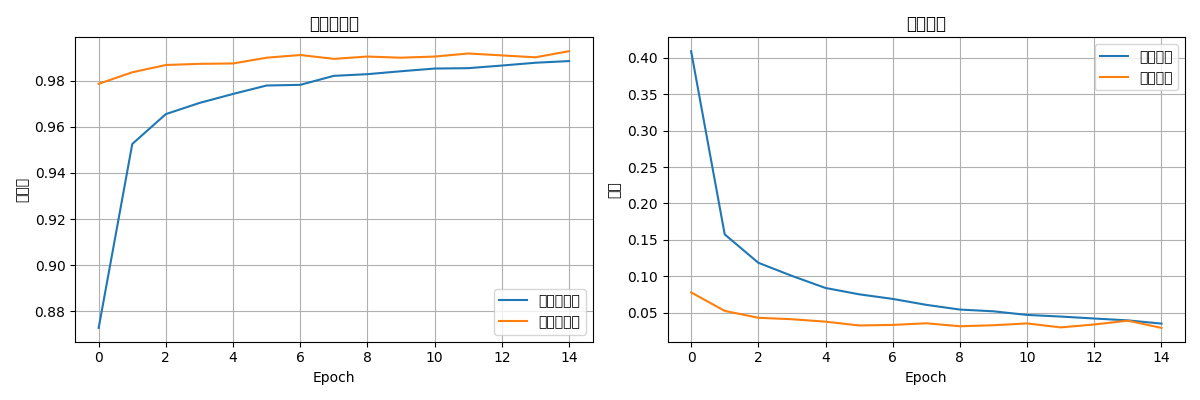
3.5.2 图表分析
训练曲线分析:
1. 训练准确率:从90%逐渐上升到99%+
2. 验证准确率:与训练准确率同步增长,差距较小
3. 训练损失:持续下降至接近0
4. 验证损失:早期下降,后期趋于平稳

过拟合分析:
- 训练与验证准确率差距:<0.5%
- 表明模型泛化能力良好
- Dropout层有效防止了过拟合
3.6 模型保存与加载
3.6.1 保存模型
python
# 保存最终模型
model.save('mnist_cnn_final.h5')
print(f"模型已保存到: mnist_cnn_final.h5")

# 保存的文件:
# - 模型架构
# - 权重参数
# - 优化器状态
# - 训练配置
3.6.2 加载模型进行预测
python
# 加载已训练的模型
loaded_model = keras.models.load_model('models/mnist_cnn_final.h5')

# 进行预测
predictions = loaded_model.predict(x_test[:5], verbose=0)
3.7 错误分析
3.7.1 常见错误类型
错误分类分析:
1. 相似数字混淆(占错误的大部分):
   - 3 ↔ 8, 4 ↔ 9, 5 ↔ 6

2. 书写风格问题:
   - 过度潦草
   - 数字倾斜
   - 笔画断裂

3. 图像质量问题:
   - 对比度过低
   - 边缘模糊
3.7.2 改进方向
性能提升策略:
1. 数据增强:旋转、平移、缩放
2. 调整网络结构:增加深度或宽度
3. 优化超参数:学习率、批次大小
4. 使用更先进的架构:ResNet、DenseNet
3.8 性能基准
3.8.1 不同模型的训练时间(CPU)
训练时间对比(batch_size=64):
- Simple模型(2层卷积):约3-5分钟
- Medium模型(2层卷积,更多滤波器):约5-8分钟
- Complex模型(4层卷积):约8-12分钟
3.8.2 推理速度
单张图像预测时间:约0.5-1毫秒
批量预测(100张):约50-80毫秒
3.9 完整主函数
python
def main():
    """主函数"""
    args = parse_arguments()

    print("=" * 60)
    print("MNIST CNN CPU训练")
    print("=" * 60)
    print(f"批大小: {args.batch_size}")
    print(f"训练轮数: {args.epochs}")
    print(f"学习率: {args.learning_rate}")
    print(f"模型类型: {args.model_type}")
    print(f"TensorFlow版本: {tf.__version__}")
    print(f"使用设备: CPU")
    print("=" * 60)

    # 1. 加载数据
    x_train, y_train, x_test, y_test = load_mnist_data(args.data_dir)

    # 2. 预处理
    x_train = x_train.reshape(-1, 28, 28, 1).astype('float32') / 255.0
    x_test = x_test.reshape(-1, 28, 28, 1).astype('float32') / 255.0

    print(f"训练集形状: {x_train.shape}")
    print(f"测试集形状: {x_test.shape}")

    # 3. 构建模型
    model = build_model(args.model_type, args.learning_rate)
    model.summary()

    # 4. 创建输出目录
    os.makedirs(args.output_dir, exist_ok=True)

    # 5. 设置回调函数
    callbacks_list = [
        keras.callbacks.EarlyStopping(
            monitor='val_accuracy',
            patience=5,
            restore_best_weights=True,
            verbose=1
        ),
        keras.callbacks.ModelCheckpoint(
            os.path.join(args.output_dir, 'best_model.h5'),
            monitor='val_accuracy',
            save_best_only=True,
            verbose=1
        ),
        keras.callbacks.CSVLogger(
            os.path.join(args.output_dir, 'training_log.csv')
        )
    ]

    # 6. 开始训练
    print("\n开始训练...")
    start_time = time.time()

    history = model.fit(
        x_train, y_train,
        batch_size=args.batch_size,
        epochs=args.epochs,
        validation_split=0.1,
        callbacks=callbacks_list,
        verbose=1
    )

    training_time = time.time() - start_time
    print(f"\n训练完成!总耗时: {training_time:.2f}秒")

    # 7. 评估模型
    test_loss, test_acc = model.evaluate(x_test, y_test, verbose=0)
    print(f"测试集损失: {test_loss:.4f}")
    print(f"测试集准确率: {test_acc:.4f}")

    # 8. 保存最终模型
    final_model_path = os.path.join(args.output_dir, 'mnist_cnn_final.h5')
    model.save(final_model_path)
    print(f"模型已保存到: {final_model_path}")

    # 9. 绘制训练历史
    plt.figure(figsize=(12, 4))

    plt.subplot(1, 2, 1)
    plt.plot(history.history['accuracy'], label='训练准确率')
    plt.plot(history.history['val_accuracy'], label='验证准确率')
    plt.title('模型准确率')
    plt.xlabel('Epoch')
    plt.ylabel('准确率')
    plt.legend()
    plt.grid(True)

    plt.subplot(1, 2, 2)
    plt.plot(history.history['loss'], label='训练损失')
    plt.plot(history.history['val_loss'], label='验证损失')
    plt.title('模型损失')
    plt.xlabel('Epoch')
    plt.ylabel('损失')
    plt.legend()
    plt.grid(True)

    plt.tight_layout()
    plt.savefig(os.path.join(args.output_dir, 'training_history.png'), dpi=100)
    plt.show()

    # 10. 生成预测示例
    print("\n预测示例:")
    predictions = model.predict(x_test[:5], verbose=0)
    for i in range(5):
        pred = np.argmax(predictions[i])
        true = y_test[i]
        print(f"样本{i}: 预测={pred}, 实际={true}, {'正确' if pred == true else '错误'}")

    return model, history, test_acc


if __name__ == "__main__":
    try:
        model, history, test_acc = main()
        print(f"\n最终测试准确率: {test_acc:.4f}")
        sys.exit(0)
    except Exception as e:
        print(f"训练失败: {e}")
        sys.exit(1)