在学习深度学习框架时,调用nn.LSTM往往只是一行代码,但理解其内部门控机制与矩阵运算才能真正掌握序列建模的本质。本文将从头实现长短期记忆网络(LSTM)的前向传播,深入解析输入门、遗忘门、输出门的计算细节,并与PyTorch官方实现进行对比验证。
一、LSTM基础原理
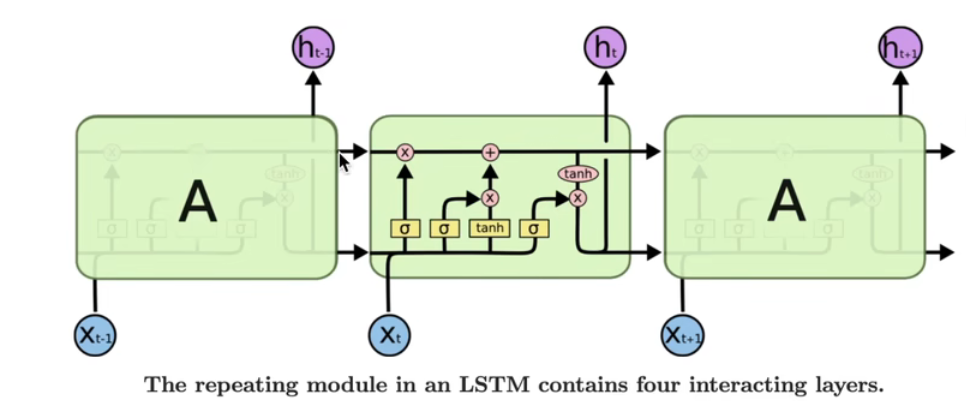
LSTM(Long Short-Term Memory)通过引入细胞状态(Cell State)和三个门控机制(输入门、遗忘门、输出门)来解决传统RNN的长期依赖问题。
核心公式
LSTM的计算流程可分为四个门控计算 和两种状态更新:
四个门控: i t = σ ( W i i x t + b i i + W h i h t − 1 + b h i ) // 输入门 f t = σ ( W i f x t + b i f + W h f h t − 1 + b h f ) // 遗忘门 g t = tanh ( W i g x t + b i g + W h g h t − 1 + b h g ) // 候选细胞状态 o t = σ ( W i o x t + b i o + W h o h t − 1 + b h o ) // 输出门 两种状态更新: c t = f t ⊙ c t − 1 + i t ⊙ g t // 细胞状态更新 h t = o t ⊙ tanh ( c t ) // 隐藏状态输出 \begin{aligned} \text{四个门控:} \\ i_t &= \sigma(W_{ii}x_t + b_{ii} + W_{hi}h_{t-1} + b_{hi}) \quad \text{// 输入门} \\ f_t &= \sigma(W_{if}x_t + b_{if} + W_{hf}h_{t-1} + b_{hf}) \quad \text{// 遗忘门} \\ g_t &= \tanh(W_{ig}x_t + b_{ig} + W_{hg}h_{t-1} + b_{hg}) \quad \text{// 候选细胞状态} \\ o_t &= \sigma(W_{io}x_t + b_{io} + W_{ho}h_{t-1} + b_{ho}) \quad \text{// 输出门} \\ \text{两种状态更新:} \\ c_t &= f_t \odot c_{t-1} + i_t \odot g_t \quad \text{// 细胞状态更新} \\ h_t &= o_t \odot \tanh(c_t) \quad \text{// 隐藏状态输出} \end{aligned} 四个门控:itftgtot两种状态更新:ctht=σ(Wiixt+bii+Whiht−1+bhi)// 输入门=σ(Wifxt+bif+Whfht−1+bhf)// 遗忘门=tanh(Wigxt+big+Whght−1+bhg)// 候选细胞状态=σ(Wioxt+bio+Whoht−1+bho)// 输出门=ft⊙ct−1+it⊙gt// 细胞状态更新=ot⊙tanh(ct)// 隐藏状态输出
其中:
- h t h_t ht:时刻 t t t 的隐藏状态(Hidden State)
- c t c_t ct:时刻 t t t 的细胞状态(Cell State),LSTM的核心记忆载体
- x t x_t xt:时刻 t t t 的输入特征
- i t , f t , o t i_t, f_t, o_t it,ft,ot:输入门、遗忘门、输出门,通过Sigmoid激活输出0-1之间的值控制信息流动
- g t g_t gt:候选记忆内容,通过Tanh激活
- ⊙ \odot ⊙:Hadamard积(逐元素乘积)
门控机制图解:
- 遗忘门 f t f_t ft:决定从细胞状态中丢弃哪些信息(0表示完全遗忘,1表示完全保留)
- 输入门 i t i_t it:决定哪些新信息存入细胞状态
- 输出门 o t o_t ot:决定基于细胞状态输出哪些隐藏状态
二、PyTorch LSTM参数详解
在实现之前,先理解PyTorch API的设计逻辑:
核心参数:
- input_size -- 输入 x x x 中预期特征的数量(输入特征维度 H i n H_{in} Hin)
- hidden_size -- 隐藏状态 h h h 和细胞状态 c c c 中的特征数量( H o u t H_{out} Hout / H c e l l H_{cell} Hcell)
- num_layers -- 循环层的数量。例如
num_layers=2表示堆叠两个LSTM,第二层接收第一层的隐藏状态作为输入。默认值:1 - bias -- 如果为
False,则不使用偏置 b i h b_{ih} bih 和 b h h b_{hh} bhh。默认值:True - batch_first -- 如果为
True,输入输出张量格式为(batch, seq, feature)而非(seq, batch, feature)。注意:这不适用于隐藏状态和细胞状态。默认值:False - dropout -- 如果非零,在除最后一层外的每个LSTM层输出上引入Dropout层。默认值:
0 - bidirectional -- 如果为
True,则变为双向LSTM。默认值:False - proj_size -- 如果大于
0,将使用对应大小的投影LSTM, h t h_t ht维度将从hidden_size变为proj_size。默认值:0
输入:input, (h_0, c_0)
-
input: 张量形状:
- 无batch输入: ( L , H i n ) (L, H_{in}) (L,Hin)
batch_first=False时: ( L , N , H i n ) (L, N, H_{in}) (L,N,Hin),即(seq, batch, feature)batch_first=True时: ( N , L , H i n ) (N, L, H_{in}) (N,L,Hin),即(batch, seq, feature)
-
h_0 : 初始隐藏状态,形状为 ( D × num_layers , N , H o u t ) (D \times \text{num\layers}, N, H{out}) (D×num_layers,N,Hout)(批处理情况)
-
c_0 : 初始细胞状态,形状为 ( D × num_layers , N , H c e l l ) (D \times \text{num\layers}, N, H{cell}) (D×num_layers,N,Hcell)
其中:
N = batch size(批量大小) L = sequence length(序列长度) D = 2 如果 bidirectional=True,否则为 1 H i n = input_size H c e l l = hidden_size H o u t = 如果 proj_size>0 则为 proj_size,否则为 hidden_size \begin{aligned} N &= \text{batch size(批量大小)} \\ L &= \text{sequence length(序列长度)} \\ D &= 2 \text{ 如果 bidirectional=True,否则为 } 1 \\ H_{in} &= \text{input\size} \\ H{cell} &= \text{hidden\size} \\ H{out} &= \text{如果 proj\_size>0 则为 proj\_size,否则为 hidden\_size} \end{aligned} NLDHinHcellHout=batch size(批量大小)=sequence length(序列长度)=2 如果 bidirectional=True,否则为 1=input_size=hidden_size=如果 proj_size>0 则为 proj_size,否则为 hidden_size
输出:output, (h_n, c_n)
-
output : 包含LSTM最后一层每个时间步的输出特征 h t h_t ht,形状与input对应:
batch_first=False时: ( L , N , D × H o u t ) (L, N, D \times H_{out}) (L,N,D×Hout)batch_first=True时: ( N , L , D × H o u t ) (N, L, D \times H_{out}) (N,L,D×Hout)
-
h_n : 最终隐藏状态,形状 ( D × num_layers , N , H o u t ) (D \times \text{num\layers}, N, H{out}) (D×num_layers,N,Hout)
-
c_n : 最终细胞状态,形状 ( D × num_layers , N , H c e l l ) (D \times \text{num\layers}, N, H{cell}) (D×num_layers,N,Hcell)
三、手撕LSTM单层实现
首先准备数据,并调用PyTorch官方API作为对比基准:
python
import torch
import torch.nn as nn

# 定义常量
batch_size, sequence_len, input_size, hidden_size = 2, 3, 4, 5

# 构造输入input和初始状态c0, h0
input = torch.randn(batch_size, sequence_len, input_size)  # [B, L, Hin]
c0 = torch.randn(batch_size, hidden_size)                  # [B, Hout]
h0 = torch.randn(batch_size, hidden_size)                  # [B, Hout]

# 调用官方API
lstm_layer = nn.LSTM(input_size, hidden_size, batch_first=True)
output, (h_final, c_final) = lstm_layer(
    input,
    (h0.unsqueeze(0), c0.unsqueeze(0))  # 官方API要求 [num_layers, B, Hout]
)

# 官方API输出维度:
# output: [B, L, Hout]
# h_final: [1, B, Hout]
# c_final: [1, B, Hout]查看官方参数组织方式:
python
for k, v in lstm_layer.named_parameters():
    print(k, v.shape)

# 输出:
# weight_ih_l0 torch.Size([20, 4])   # [4*Hout, Hin]
# weight_hh_l0 torch.Size([20, 5])   # [4*Hout, Hout]
# bias_ih_l0 torch.Size([20])        # [4*Hout]
# bias_hh_l0 torch.Size([20]) # [4*Hout]关键理解:PyTorch将四个门的权重矩阵拼接存储:
weight_ih= W i i ; W i f ; W i g ; W i o W_{ii}; W_{if}; W_{ig}; W_{io} Wii;Wif;Wig;Wio(按行拼接,形状 4 × H o u t , H i n 4\\times H_{out}, H_{in} 4×Hout,Hin)weight_hh= W h i ; W h f ; W h g ; W h o W_{hi}; W_{hf}; W_{hg}; W_{ho} Whi;Whf;Whg;Who(形状 4 × H o u t , H o u t 4\\times H_{out}, H_{out} 4×Hout,Hout)bias_ih= b i i ; b i f ; b i g ; b i o b_{ii}; b_{if}; b_{ig}; b_{io} bii;bif;big;bio(形状 4 × H o u t 4\\times H_{out} 4×Hout)bias_hh= b h i ; b h f ; b h g ; b h o b_{hi}; b_{hf}; b_{hg}; b_{ho} bhi;bhf;bhg;bho(形状 4 × H o u t 4\\times H_{out} 4×Hout)
接下来是核心------手动实现LSTM前向传播:
python
def lstm_forward(input, initial_states, w_ih, w_hh, b_ih, b_hh):
    """
    手动实现LSTM前向传播

    Args:
        input: [B, L, Hin]
        initial_states: (h0, c0),每个都是 [B, Hout]
        w_ih: [4*Hout, Hin],输入到隐藏层的权重
        w_hh: [4*Hout, Hout],隐藏层到隐藏层的循环权重
        b_ih, b_hh: [4*Hout],偏置项
    """
    h0, c0 = initial_states
    batch_size, sequence_len, input_size = input.shape
    hidden_size = w_ih.shape[0] // 4  # 因为是四个门的权重拼接

    prev_h = h0  # [B, Hout]
    prev_c = c0  # [B, Hout]

    # 为批次并行计算准备权重矩阵:扩展batch维度
    # w_ih: [4*Hout, Hin] -> [B, 4*Hout, Hin]
    batch_w_ih = w_ih.unsqueeze(0).tile(batch_size, 1, 1)
    # w_hh: [4*Hout, Hout] -> [B, 4*Hout, Hout]
    batch_w_hh = w_hh.unsqueeze(0).tile(batch_size, 1, 1)

    # 初始化输出序列 [B, L, Hout]
    output = torch.zeros(batch_size, sequence_len, hidden_size)

    # 遍历时间步
    for t in range(sequence_len):
        x = input[:, t, :]  # 获取当前时刻输入 [B, Hin]

        # 计算 w_ih @ x: [B, 4*Hout, Hin] @ [B, Hin, 1] -> [B, 4*Hout, 1]
        w_times_x = torch.bmm(batch_w_ih, x.unsqueeze(2)).squeeze(-1)  # [B, 4*Hout]

        # 计算 w_hh @ h_{t-1}: [B, 4*Hout, Hout] @ [B, Hout, 1] -> [B, 4*Hout]
        w_times_h_prev = torch.bmm(batch_w_hh, prev_h.unsqueeze(2)).squeeze(-1)  # [B, 4*Hout]

        # 分别计算四个门(通过切片获取对应权重部分)
        # 输入门 i_t
        i_t = torch.sigmoid(
            w_times_x[:, :hidden_size] +
            w_times_h_prev[:, :hidden_size] +
            b_ih[:hidden_size].unsqueeze(0).tile(batch_size, 1) +
            b_hh[:hidden_size].unsqueeze(0).tile(batch_size, 1)
        )  # [B, Hout]

        # 遗忘门 f_t
        f_t = torch.sigmoid(
            w_times_x[:, hidden_size:2*hidden_size] +
            w_times_h_prev[:, hidden_size:2*hidden_size] +
            b_ih[hidden_size:2*hidden_size].unsqueeze(0).tile(batch_size, 1) +
            b_hh[hidden_size:2*hidden_size].unsqueeze(0).tile(batch_size, 1)
        )  # [B, Hout]

        # 候选细胞状态 g_t
        g_t = torch.tanh(
            w_times_x[:, 2*hidden_size:3*hidden_size] +
            w_times_h_prev[:, 2*hidden_size:3*hidden_size] +
            b_ih[2*hidden_size:3*hidden_size].unsqueeze(0).tile(batch_size, 1) +
            b_hh[2*hidden_size:3*hidden_size].unsqueeze(0).tile(batch_size, 1)
        )  # [B, Hout]

        # 输出门 o_t
        o_t = torch.sigmoid(
            w_times_x[:, 3*hidden_size:] +
            w_times_h_prev[:, 3*hidden_size:] +
            b_ih[3*hidden_size:].unsqueeze(0).tile(batch_size, 1) +
            b_hh[3*hidden_size:].unsqueeze(0).tile(batch_size, 1)
        )  # [B, Hout]

        # 细胞状态更新:c_t = f_t * c_{t-1} + i_t * g_t
        prev_c = f_t * prev_c + i_t * g_t  # [B, Hout]

        # 隐藏状态输出:h_t = o_t * tanh(c_t)
        prev_h = o_t * torch.tanh(prev_c)  # [B, Hout]

        # 存储当前时刻输出
        output[:, t, :] = prev_h

    return output, (prev_h, prev_c)
四、关键实现细节解析
1. 权重矩阵的批次并行(bmm)
为了实现批次数据的并行计算,需要将权重矩阵扩展到批次维度:
python
batch_w_ih = w_ih.unsqueeze(0).tile(batch_size, 1, 1) # [1, 4*Hout, Hin] -> [B, 4*Hout, Hin]这样每个样本都使用相同的权重进行独立计算,通过torch.bmm(批次矩阵乘法)实现高效并行。
2. 维度对齐技巧
- 输入 x t x_t xt 初始形状
[B, Hin],通过unsqueeze(2)变为[B, Hin, 1],便于与权重[B, 4*Hout, Hin]进行矩阵乘法 - 结果
[B, 4*Hout, 1]通过squeeze(-1)压缩回[B, 4*Hout],便于后续门控计算
3. 四权重拼接的切片访问
PyTorch将四个门的权重拼接存储,因此通过切片获取:
python
# 第0~Hout行:输入门权重
# 第Hout~2*Hout行:遗忘门权重
# 第2*Hout~3*Hout行:候选状态权重
# 第3*Hout~4*Hout行:输出门权重
4. 偏置的广播机制
由于PyTorch存储的偏置是1维[4*Hout],需要扩展为[B, Hout]以进行批次加法:
python
b_ih[:hidden_size].unsqueeze(0).tile(batch_size, 1) # [Hout] -> [1, Hout] -> [B, Hout]五、验证实现正确性
使用官方API的参数测试手写实现:
python
# 提取官方LSTM的参数
w_ih = lstm_layer.weight_ih_l0
w_hh = lstm_layer.weight_hh_l0
b_ih = lstm_layer.bias_ih_l0
b_hh = lstm_layer.bias_hh_l0

# 调用自定义实现
custom_output, (custom_h_final, custom_c_final) = lstm_forward(
    input, (h0, c0), w_ih, w_hh, b_ih, b_hh
)

print("PyTorch API nn.LSTM output:")
print(output, h_final.squeeze(0), c_final.squeeze(0))
print("\ncustom lstm_forward() output:")
print(custom_output, custom_h_final, custom_c_final)

# 数值对比(应几乎完全相同,误差在1e-6级别)
print("\nDifference:", torch.abs(output - custom_output).max())
验证结果 :若两者输出一致(误差小于 10 − 6 10^{-6} 10−6),说明我们的数学推导和实现逻辑与PyTorch底层C++实现完全吻合。
六、LSTM的优缺点总结
LSTM的优点:
- 有效解决RNN的长期依赖问题(梯度消失/爆炸),可记忆数十到数百个时间步的信息
- 通过门控机制精确控制信息的遗忘与更新,适合长序列建模(如文本生成、时间序列预测)
- 细胞状态 c t c_t ct 的线性传递(累加操作)提供了稳定的梯度传播路径
LSTM的缺点:
- 计算复杂度高:每个时间步需要计算4个门控,参数量是标准RNN的4倍
- 串行计算无法并行化时间步,推理速度较慢
- 内存占用大:需要同时保存 h t h_t ht和 c t c_t ct两个状态向量
七、总结
通过手撕LSTM的实现,我们深入理解了:
- 门控机制:输入门、遗忘门、输出门如何协同工作,通过Sigmoid控制信息流动比例,Tanh生成候选内容
- 双状态设计 :细胞状态 c t c_t ct作为长期记忆载体(线性更新),隐藏状态 h t h_t ht作为短期输出(非线性变换)
- 矩阵拼接:理解PyTorch将四组权重拼接存储的工程实践,掌握张量切片与维度对齐技巧
- 批次并行 :使用
bmm实现多样本并行计算,理解unsqueeze/squeeze在维度对齐中的作用
虽然实际项目中直接使用nn.LSTM即可,但这种底层实现训练有助于理解:
- 梯度裁剪在LSTM中的必要性
- 双向LSTM的实现原理(正反向各一个LSTM,输出拼接)
- 多层堆叠LSTM的实现(上一层的 h t h_t ht作为下一层的 x t x_t xt)
- 变长序列的PackedSequence处理
完整代码已验证:上述代码可直接运行,输出结果与PyTorch官方API完全一致,证明我们的实现正确复现了LSTM的门控逻辑与矩阵运算流程。
注:对于带投影的LSTM(proj_size > 0),只需在输出时增加 h t = W h r h t h_t = W_{hr}h_t ht=Whrht 的线性投影步骤,将维度从hidden_size映射到proj_size,其余逻辑完全一致。