深度学习笔记三

一、神经网络中的偏差与方差

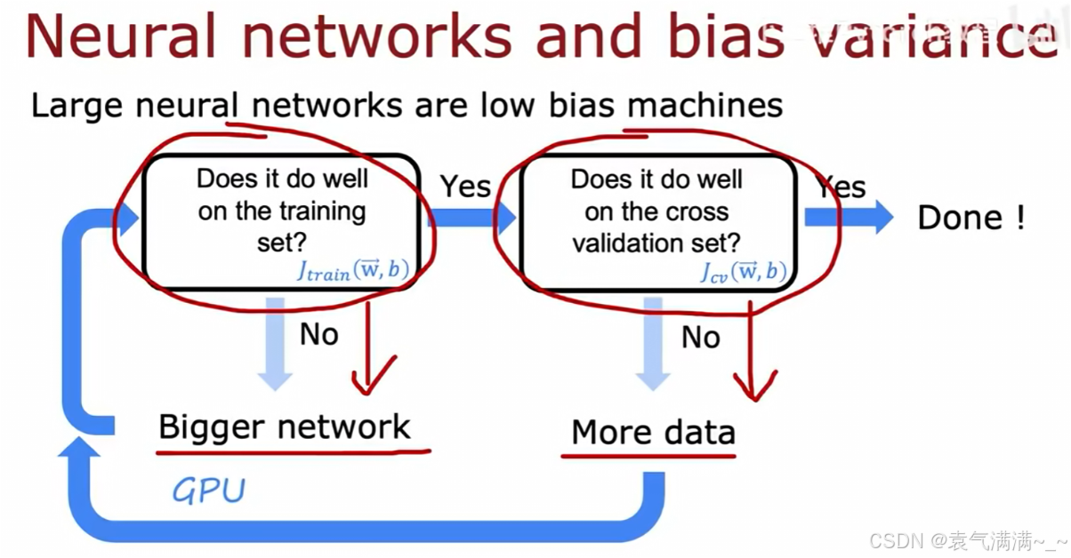
检查训练集表现。判断是否足够低。
- 如果"否"（很高），说明模型存在高偏差问题(欠拟合)。解决方案是使用一个更大的网络（增加层数或每层的神经元数量）。
- 如果"是"，检查交叉验证集表现。判断是否足够低。
  - 如果"否"（>>），说明模型存在高方差问题(过拟合)。解决方案通常是获取更多的数据。
  - 如果"是"，则模型的偏差和方差都得到了很好的控制，调试完成。

在神经网络中，我们会担心网络太大导致过拟合。然而，现实表明：只要正则化选择得当，一个更大的神经网络会与一个小的网络表现得一样好，甚至更好。

python 复制代码

layer1 = Dense(units=25,activation='relu',kernel_regularizer=L2(0.01))
layer2 = Dense(units=15,activation='relu',kernel_regularizer=L2(0.01))
layer3 = Dense(units=1,activation='sigmoid',kernel_regularizer=L2(0.01))
model = Sequential([layer1,layer2,layer3])

二、数据增强

在已有数据集的基础上，通过变形数据来获取多样性从而使模型泛化能力增强。

在图片或音频数据上加入背景噪音
改变图片的颜色和形状

常见的方法：翻转、切割、变色......

python 复制代码

%matplotlib inline
import torch
import torchvision
from torch import nn
from d2l import torch as d2l

d2l.set_figsize()
img = d2l.Image.open('lena.png')
d2l.plt.imshow(img)

python 复制代码

def apply(img, aug, num_rows=2, num_cols=4, scale=1.5):# scale=1.5指图片的总显示尺寸为默认尺寸的150%
    Y = [aug(img) for _ in range(num_rows * num_cols)]
    d2l.show_images(Y, num_rows, num_cols,scale=scale)

python 复制代码

# 水平翻转
apply(img,torchvision.transforms.RandomHorizontalFlip())

python 复制代码

# 上下翻转
apply(img,torchvision.transforms.RandomVerticalFlip())

python 复制代码

# 随机裁剪
shape_aug = torchvision.transforms.RandomResizedCrop(
    (200,200),scale=(0.1,1),ratio=(0.5,2))# ratio高宽比
apply(img,shape_aug)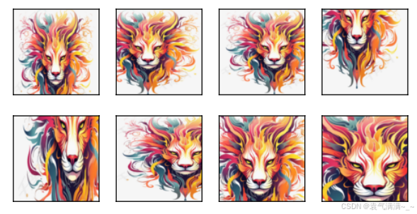

python 复制代码

# 亮度、对比度、饱和度、色温
color_aug = torchvision.transforms.ColorJitter(brightness=0.5, contrast=0.5,saturation=0.5,hue=0.5)
apply(img,color_aug)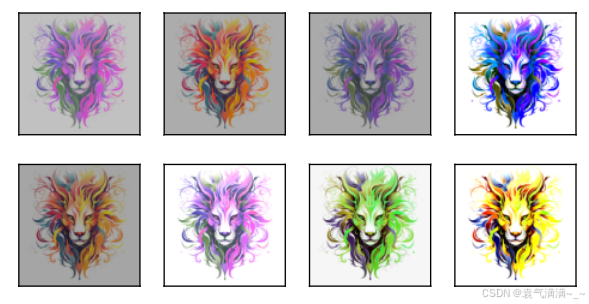

python 复制代码

# 通常而言，数据增强不只用一种方法，而是通过多种方法来增加数据多样性
aug = torchvision.transforms.Compose([
    torchvision.transforms.RandomHorizontalFlip(),
    color_aug,shape_aug])
apply(img,aug)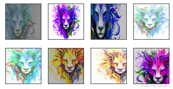

三、迁移学习和微调

一个神经网络一般可以分为两部分，一部分是特征提取，一部分是分类。

模型训练包括两种：

从头搭建模型进行训练
通过预训练模型进行训练

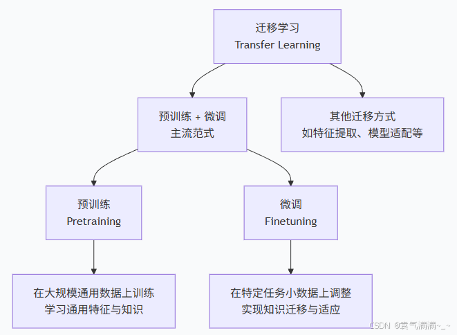
迁移学习就是把已训练好的模型参数迁移到新的模型来帮助新模型训练。

预训练是指在大量通用数据上对模型进行初步训练的过程。

微调就是利用特定领域的数据集对已预训练的大模型进行进一步训练的过程。

|-------|----------|------|-------------|
| 微调类型 | 参数更新范围 | 计算成本 | 适用场景 |
| 特征提取 | 仅最后一层 | 很低 | 数据极少，相似度高 |
| 部分微调 | 最后几层 | 中等 | 数据较少，中等相似度 |
| 全模型微调 | 所有参数 | 高 | 数据充足，任务差异大 |
| 适配器微调 | 插入的适配器参数 | 很低 | 多任务，避免灾难性遗忘 |
| ...... ||||

python 复制代码

%matplotlib inline
import os
import torch
import torchvision
from torch import nn
from d2l import torch as d2l

# 下载数据
d2l.DATA_HUB['hotdog'] = (d2l.DATA_URL+'hotdog.zip',
                          'fba480ffa8aa7e0febbb511d181409f899b9baa5')
data_dir = d2l.download_extract('hotdog')

train_img = torchvision.datasets.ImageFolder(os.path.join(data_dir,'train'))
test_img = torchvision.datasets.ImageFolder(os.path.join(data_dir,'test'))

# 查看数据
hotdogs = [train_img[i][0] for i in range(8)]
not_hotdogs = [train_img[-i-1][0] for i in range(8)]
d2l.show_images(hotdogs+not_hotdogs,2,8,scale=1.4) # 见图1

# 数据增强
normalize = torchvision.transforms.Normalize([0.485,0.456,0.406],[0.229,0.224,0.225]) # 对每个RGB通道作均值方差

train_augs = torchvision.transforms.Compose([
    torchvision.transforms.RandomResizedCrop(224),
    torchvision.transforms.RandomHorizontalFlip(),
    torchvision.transforms.ToTensor(),normalize])
test_augs = torchvision.transforms.Compose([
    torchvision.transforms.Resize(256),
    torchvision.transforms.CenterCrop(224),
    torchvision.transforms.ToTensor(),normalize])

# 下载模型
pretrained_net = torchvision.models.resnet18(pretrained=True)
pretrained_net.fc

# 微调
finetune_net = torchvision.models.resnet18(pretrained=True)
finetune_net.fc = nn.Linear(finetune_net.fc.in_features,2) # 把输出层改为线性层，in_features是512，类别数变为2
nn.init.xavier_uniform_(finetune_net.fc.weight) # 对输出层的weight作随机初始化

# 如果param_group=True，输出层中的模型参数将使用十倍的学习率
def train_fine_tuning(net, learning_rate, batch_size=128, num_epochs=5,
                      param_group=True):
    train_iter = torch.utils.data.DataLoader(torchvision.datasets.ImageFolder(
        os.path.join(data_dir, 'train'), transform=train_augs),
        batch_size=batch_size, shuffle=True)
    test_iter = torch.utils.data.DataLoader(torchvision.datasets.ImageFolder(
        os.path.join(data_dir, 'test'), transform=test_augs),
        batch_size=batch_size)
    devices = d2l.try_all_gpus()
    loss = nn.CrossEntropyLoss(reduction="none")
    if param_group:
        params_1x = [param for name, param in net.named_parameters()
             if name not in ["fc.weight", "fc.bias"]]
        trainer = torch.optim.SGD([{'params': params_1x},
                                   {'params': net.fc.parameters(),
                                    'lr': learning_rate * 10}],
                                lr=learning_rate, weight_decay=0.001)
    else:
        trainer = torch.optim.SGD(net.parameters(), lr=learning_rate,
                                  weight_decay=0.001)
    d2l.train_ch13(net, train_iter, test_iter, loss, trainer, num_epochs,
                   devices)

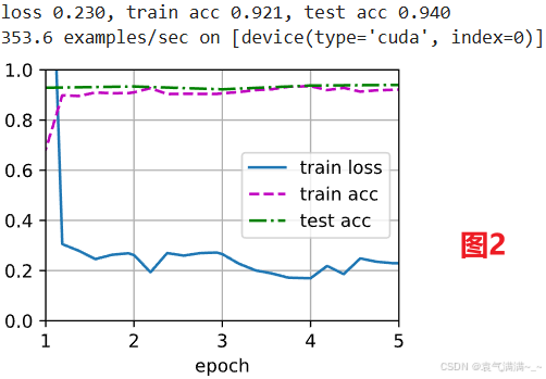
train_fine_tuning(finetune_net, 5e-5) # 见图2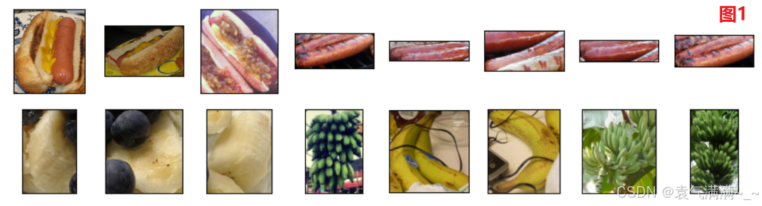

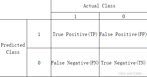
四、偏斜类别下的模型评估

当数据集中正负样本数量严重不均衡时，即存在偏斜类别（skewed classes），准确率会成为一个有误导性的评估指标。

以一个罕见病分类为例：

一个分类器 f(x) 被训练用于检测疾病（y=1 代表患病）。该分类器在测试集上达到了1%的错误率。
但该疾病在人群中的真实患病率仅为0.5%。一个不进行任何学习，只是简单地对所有人都预测y=0（健康）的程序，其错误率仅为0.5%。
这个结果（0.5%错误率）优于训练好的模型（1%错误率），这表明在偏斜类别问题中，高准确率并不能证明模型的有效性。

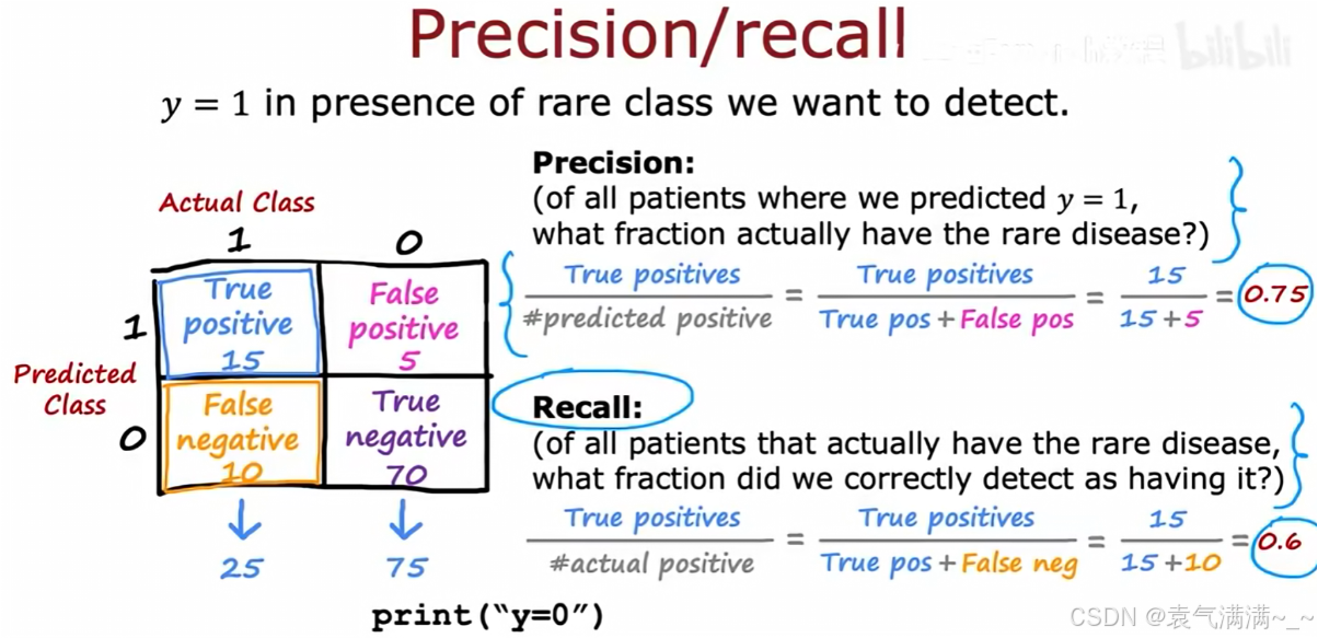
1、精确率 (Precision）

在所有被模型预测为y=1的病人中，真实患病的比例是多少
15/(15+5)=0.75

2、召回率 (Recall)

在所有真实患病的病人中，被模型成功检测出的比例是多少
15/(15+10)=0.6

3、权衡精确率和召回率

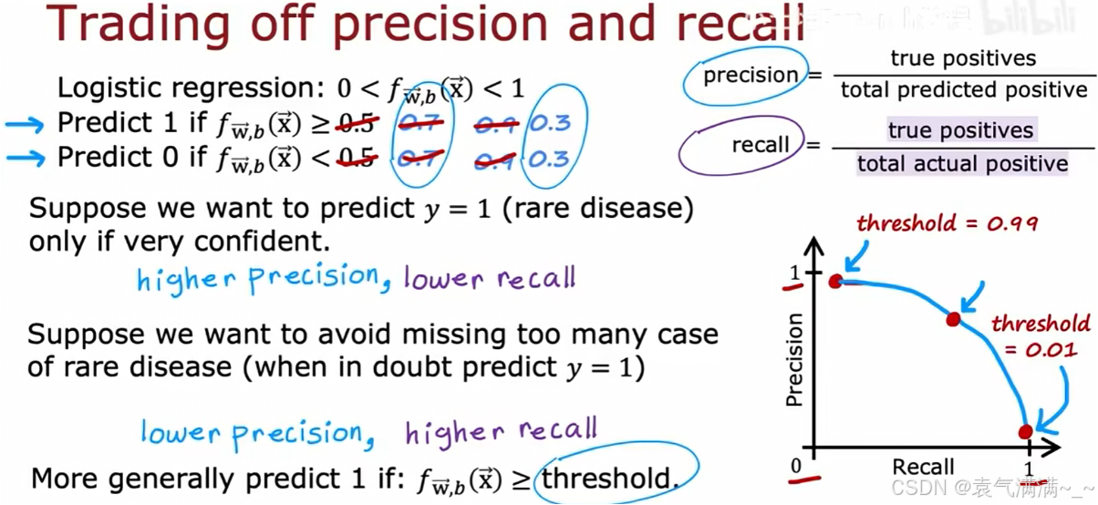
精确率和召回率之间存在权衡关系，这种关系可以通过调整分类器的阈值来控制。

逻辑回归输出一个0到1之间的概率 f(x)。预测 y=1 的条件是 f(x) >= threshold。
- 高阈值（如threshold=0.9时）：只有在模型极度确信时才预测 y=1。这会使精确率变高，召回率变低。
- 低阈值（如threshold=0.1时）：只要模型对 y=1 存在一丝可能性就进行预测。这会使召回率变高，精确率变低。

4、F1分数：综合评估指标

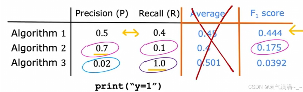
首先取P和R的平均数是不可取的，由图可得，它可能会给一个精确率极低的模型高分
所以选择F1分数，它要求P和R都比较高时，其值才会高

五、决策树

决策树（Decision Tree）是一种常用的机器学习算法，广泛应用于分类和回归问题。它通过树状结构表示决策过程，每个内部节点代表一个特征的测试，每个分支代表测试结果，每个叶节点代表一个类别或值。决策树的核心思想是递归地将数据集划分为更小的子集，直至满足停止条件。

1、模型结构

根节点：决策树的起点，包含全部训练样本，并根据最优特征进行第一次划分。
内部节点：又称中间节点，表示一个特征测试条件。每个内部节点会根据某个特征的取值将样本划分到不同的子节点。
叶结点：最终的决策结果或预测值。在分类任务中，叶节点对应一个类别标签；在回归任务中，叶节点对应一个数值预测。

从根节点到叶子节点的一条路径就是一条决策规则，可直接用于对新样本进行分类或预测。

决策树的学习是一个递归分裂（Recursive splitting的算法，其流程如下：

从根节点开始，该节点包含所有训练样本
计算所有可用特征的信息增益，选择信息增益最高的特征
根据所选特征将数据集分裂，创建新的分支和子节点
对每个子节点，递归地重复步骤2和3，直到满足预设的停止条件

停止划分的条件：

当一个节点已经是100%的同一类别时
当分裂会导致树超过预设的最大深度时
当分裂带来的纯度提升低于某个阈值时
当一个节点中的样本数量低于某个阈值时

2、用熵衡量不纯度

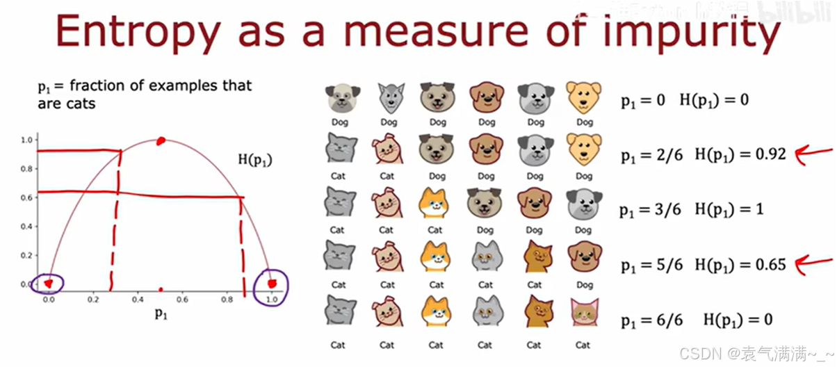
熵(Entropy)是用来衡量不纯度的常用指标。

被定义为节点中"是猫"的样本所占的比例。

熵函数的图像显示：

当节点完全纯净时（或），。
当节点最不纯时（），熵达到最大值。

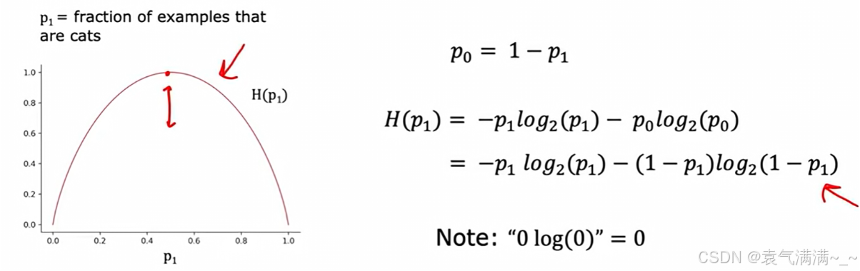
熵的计算公式 (针对二分类问题)：，其中。

3、信息增益：选择最佳的划分特征

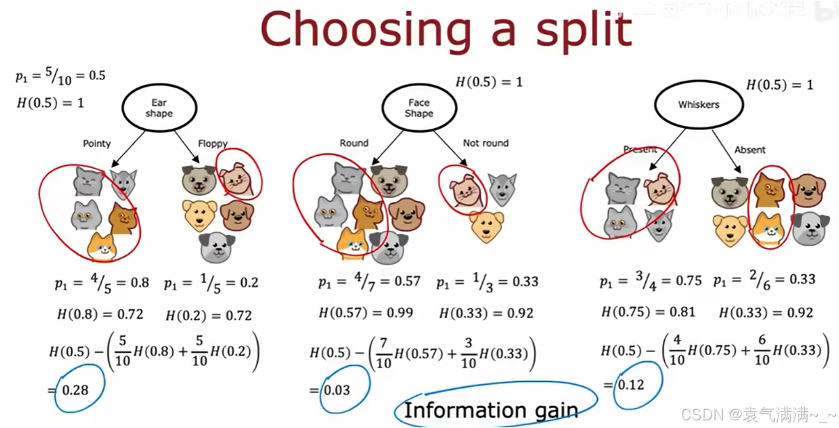
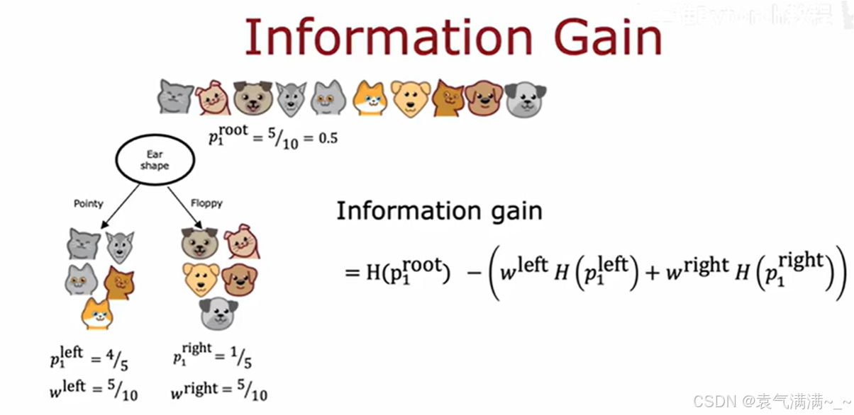
信息增益(Information Gain)是指通过某个特征对数据集进行划分后，熵减少的程度。信息增益越大，表示该特征对分类的贡献越大，通常优先选择信息增益最大的特征来构建决策树。

4、特征处理

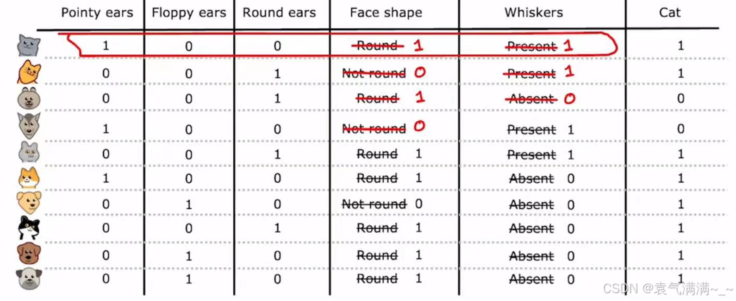
4.1 处理多值分类特征：独热编码

当一个特征有三种及以上的特征值时，我们通常采用独热编码的处理方式，处理规则如下：

如果一个分类特征有 k 个可能的取值，那么就创建 k 个新的二元特征，每个特征只取0或1。
对于一个样本，其原始特征值对应的那个新特征为1，其余 k-1 个新特征都为0。

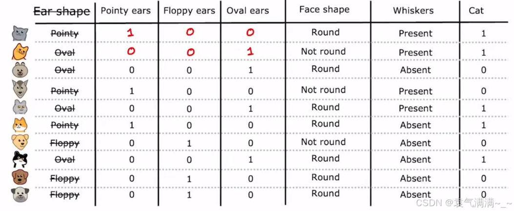
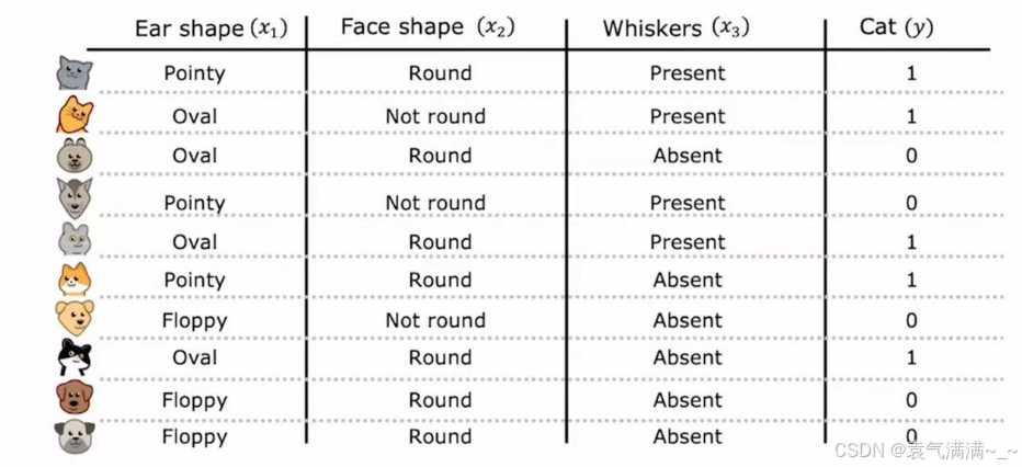
这种将分类数据转换为数值数据的技术不仅适用于决策树，也适用于神经网络等其他多种机器学习模型，因为这些模型通常期望输入是数值形式。通过独热编码，我们可以将所有分类特征（如"Face shape"、"Whiskers"）都转换为0和1的表示，从而形成一个完全由数值组成的输入数据集。

4.2 处理连续特征

除了分类特征，数据集中也常常包含连续特征，如下图的"Weight (lbs.)"。

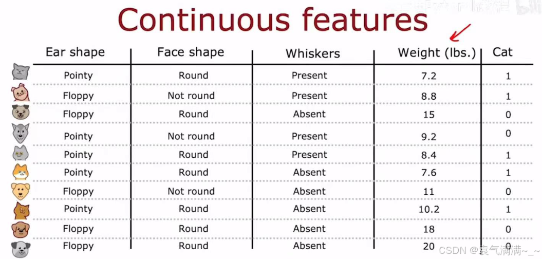
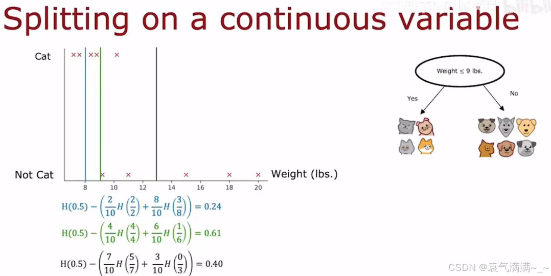
对于一个连续特征，决策树需要决定一个分割点，将其转换为一个二元判断。eg：对于体重特征，一个可能的分割是"Weight <= 9 lbs."。

决策过程：算法会尝试所有可能的分割点。
选择标准：对于每一个尝试的分割点，算法都会计算其信息增益。
最终，算法会选择最高信息增益的分割点作为这个连续特征的最佳分割策略。

六、练习

1、识别手写数字

python 复制代码

import numpy as np
import tensorflow as tf
from tensorflow.keras.models import Sequential
from tensorflow.keras.layers import Dense
from tensorflow.keras.activations import linear, relu, sigmoid
import matplotlib.pyplot as plt

X = np.load("data/X.npy")
y = np.load("data/y.npy")
print ('The shape of X is: ' + str(X.shape)) # (5000, 400)
print ('The shape of y is: ' + str(y.shape)) # (5000, 1)

tf.random.set_seed(1234) # for consistent results
model = Sequential(
    [               
        tf.keras.Input(shape=(400,)),
        Dense(units=25,activation='relu'),
        Dense(units=15,activation='relu'),
        Dense(units=10,activation='linear')
    ], name = "my_model" 
)

model.compile(
    loss=tf.keras.losses.SparseCategoricalCrossentropy(from_logits=True),
    optimizer=tf.keras.optimizers.Adam(learning_rate=0.001),
)

history = model.fit(X,y,epochs=40)

fig,ax = plt.subplots(1,1, figsize = (4,3))
ax.plot(history.history['loss'], label='loss')
ax.set_ylim([0, 2])
ax.set_xlabel('Epoch')
ax.set_ylabel('loss (cost)')
ax.legend()
ax.grid(True)
plt.show()

# 预测
image_of_two = X[1015]
fig, ax = plt.subplots(1,1, figsize=(0.5,0.5))
X_reshaped = image_of_two.reshape((20,20)).T
ax.imshow(X_reshaped, cmap='gray')
plt.show()
prediction = model.predict(image_of_two.reshape(1,400))
print(f" predicting a Two: \n{prediction}")
print(f" Largest Prediction index: {np.argmax(prediction)}") # 2

# 概率
prediction_p = tf.nn.softmax(prediction)
print(f" predicting a Two. Probability vector: \n{prediction_p}")
print(f"Total of predictions: {np.sum(prediction_p):0.3f}") # 概率之和为 1

# 返回预测目标整数
yhat = np.argmax(prediction_p)
print(f"np.argmax(prediction_p): {yhat}") # 2

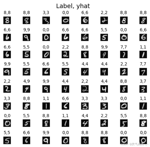
# 随机抽样64个数据进行预测
m, n = X.shape

fig, axes = plt.subplots(8,8, figsize=(5,5))
fig.tight_layout(pad=0.13,rect=[0, 0.03, 1, 0.91]) #[left, bottom, right, top]
for i,ax in enumerate(axes.flat):
    # Select random indices
    random_index = np.random.randint(m)
    
    # Select rows corresponding to the random indices and
    # reshape the image
    X_random_reshaped = X[random_index].reshape((20,20)).T
    
    # Display the image
    ax.imshow(X_random_reshaped, cmap='gray')
    
    # Predict using the Neural Network
    prediction = model.predict(X[random_index].reshape(1,400))
    prediction_p = tf.nn.softmax(prediction)
    yhat = np.argmax(prediction_p)
    
    # Display the label above the image
    ax.set_title(f"{y[random_index,0]},{yhat}",fontsize=10)
    ax.set_axis_off()
fig.suptitle("Label, yhat", fontsize=14)
plt.show()

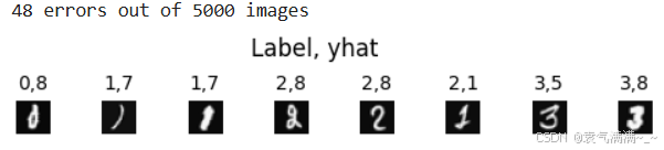
# 检查错误
f = model.predict(X)
yhat = np.argmax(f, axis=1)
doo = yhat != y[:,0]
idxs = np.where(yhat != y[:,0])[0]
if len(idxs) == 0:
    print("no errors found")
else:
    cnt = min(8, len(idxs))
    fig, ax = plt.subplots(1,cnt, figsize=(5,1.2))
    fig.tight_layout(pad=0.13,rect=[0, 0.03, 1, 0.80]) #[left, bottom, right, top]

    for i in range(cnt):
        j = idxs[i]
        X_reshaped = X[j].reshape((20,20)).T

        ax[i].imshow(X_reshaped, cmap='gray')

        prediction = model.predict(X[j].reshape(1,400))
        prediction_p = tf.nn.softmax(prediction)
        yhat = np.argmax(prediction_p)

        ax[i].set_title(f"{y[j,0]},{yhat}",fontsize=10)
        ax[i].set_axis_off()
        fig.suptitle("Label, yhat", fontsize=12)
print( f"{len(idxs)} errors out of {len(X)} images")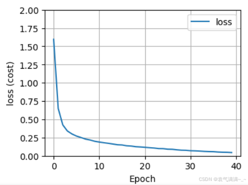

2、通过决策树分类器对鸢尾花（Iris）数据集进行分类任务

python 复制代码

from sklearn.datasets import load_iris
from sklearn.model_selection import train_test_split
from sklearn.tree import DecisionTreeClassifier
from sklearn.metrics import accuracy_score

# 加载鸢尾花数据集
iris = load_iris()
X = iris.data
y = iris.target

# 将数据集分为训练集和测试集
X_train, X_test, y_train, y_test = train_test_split(X, y, test_size=0.3, random_state=42)

# 创建决策树分类器
clf = DecisionTreeClassifier()

# 训练模型
clf.fit(X_train, y_train)

# 对测试集进行预测
y_pred = clf.predict(X_test)

# 计算准确率
accuracy = accuracy_score(y_test, y_pred)
print(f"模型准确率: {accuracy:.2f}")