多元回归的本质和一元回归是一样的,但本文希望以此引入矩阵表达,来作为一种通用的形式。此外,由于上午已经介绍过小批量梯度下降是目前深度学习中应用最广泛的,因此在之后的文章中,都会才会此方法。
通过本文,希望能理解多元线性回归的数学原理,并讨论不同批量大小对收敛的影响
原理介绍
多元线性回归模型
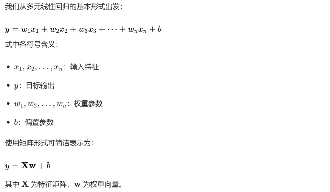
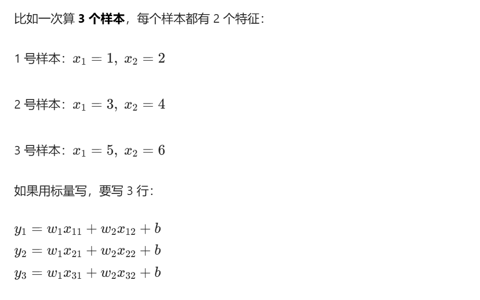
为什么可以这样表达(以2特征为例)
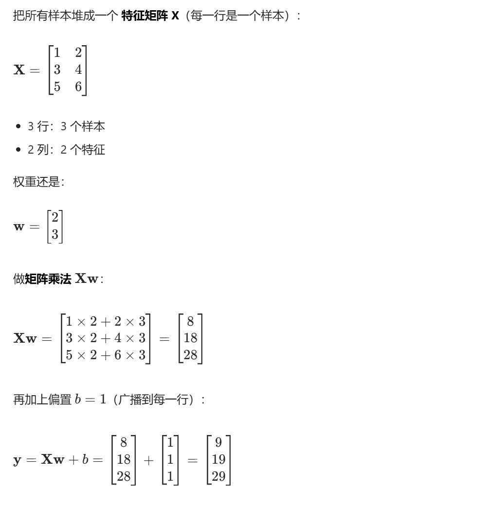
如果尝试用矩阵表达呢?
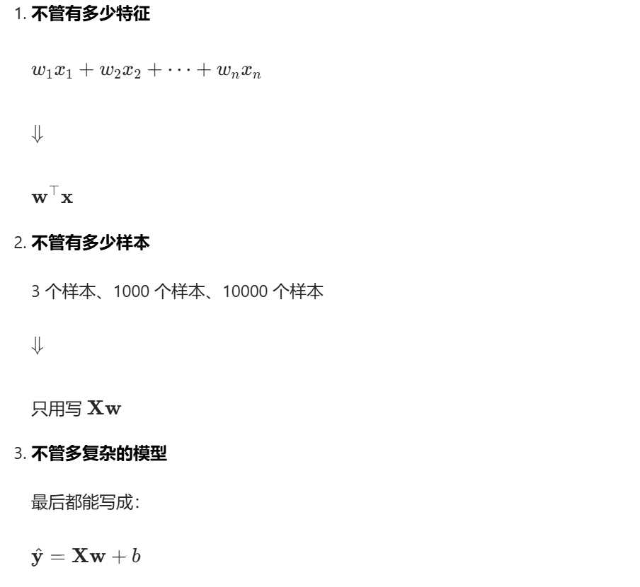
由此我们可以总结
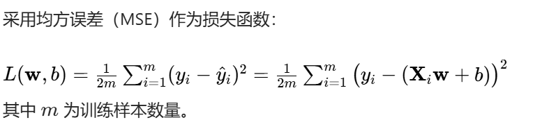
损失函数
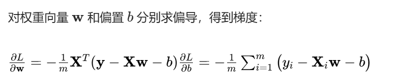
梯度计算
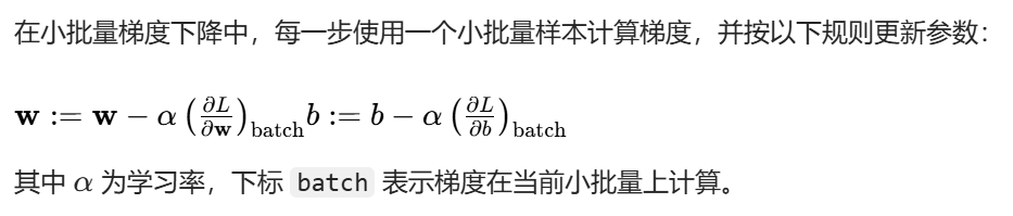
小批量梯度下降更新规则
代码实现
1、数据生成
我们将生成一个包含三个特征的合成数据集,模拟真实多元线性关系,并添加一些噪声来模拟真实情况。
python
# 设置随机种子保证结果可重现
np.random.seed(42)

# 生成数据集
m = 500  # 样本数量
n_features = 3  # 特征数量

# 真实参数
true_w = np.array([2.5, -1.8, 3.2])  # 权重
true_b = 1.0  # 偏置

# 生成输入特征 X (m x n_features)
X = np.random.uniform(-5, 5, (m, n_features))

# 生成目标值 y = X @ true_w + true_b + 噪声
noise = np.random.normal(0, 0.5, m)  # 添加高斯噪声
y = X @ true_w + true_b + noise

# 可视化数据分布
fig = plt.figure(figsize=(15, 5))

# 特征分布
for i in range(n_features):
    plt.subplot(1, 4, i+1)
    plt.hist(X[:, i], bins=30, alpha=0.7, color=f'C{i}')
    plt.xlabel(f'x{i+1}')
    plt.ylabel('频次')
    plt.title(f'特征 x{i+1} 分布')
    plt.grid(True, alpha=0.3)

# 目标值分布
plt.subplot(1, 4, 4)
plt.hist(y, bins=30, alpha=0.7, color='red')
plt.xlabel('y')
plt.ylabel('频次')
plt.title('目标值 y 分布')
plt.grid(True, alpha=0.3)

plt.tight_layout()
plt.show()

print(f"数据集大小: {m} 个样本")
print(f"特征数量: {n_features}")
print(f"真实参数: w = {true_w}, b = {true_b}")
print(f"X 范围: [{X.min():.2f}, {X.max():.2f}]")
print(f"y 范围: [{y.min():.2f}, {y.max():.2f}]")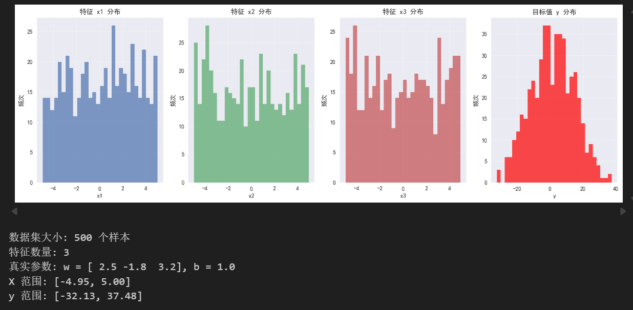
2、实现损失函数与梯度计算
这里与上一篇文章中的内容基本一样,只是需要更新的参数多了一些
python
def compute_loss(w, b, X, y):
    """
    计算均方误差损失函数

    参数:
    w: 权重向量 (n_features,)
    b: 偏置标量
    X: 特征矩阵 (m, n_features)
    y: 目标向量 (m,)

    返回:
    loss: 损失值
    """
    m = len(X)
    y_pred = X @ w + b
    loss = (1/(2*m)) * np.sum((y - y_pred)**2)
    return loss

def compute_gradients(w, b, X, y):
    """
    计算损失函数对参数的梯度

    参数:
    w: 权重向量 (n_features,)
    b: 偏置标量
    X: 特征矩阵 (m, n_features)
    y: 目标向量 (m,)

    返回:
    dw: 权重梯度 (n_features,)
    db: 偏置梯度 (标量)
    """
    m = len(X)
    y_pred = X @ w + b
    error = y - y_pred

    dw = -(1/m) * X.T @ error
    db = -(1/m) * np.sum(error)

    return dw, db

def compute_batch_gradients(w, b, X_batch, y_batch):
    """
    计算小批量上的梯度

    参数:
    w: 权重向量 (n_features,)
    b: 偏置标量
    X_batch: 小批量特征矩阵 (batch_size, n_features)
    y_batch: 小批量目标向量 (batch_size,)

    返回:
    dw: 权重梯度 (n_features,)
    db: 偏置梯度 (标量)
    """
    batch_size = len(X_batch)
    y_pred = X_batch @ w + b
    error = y_batch - y_pred

    dw = -(1/batch_size) * X_batch.T @ error
    db = -(1/batch_size) * np.sum(error)

    return dw, db

# 测试函数
w_test = np.array([1.0, 0.5, -0.5])
b_test = 0.0
loss_test = compute_loss(w_test, b_test, X, y)
dw_test, db_test = compute_gradients(w_test, b_test, X, y)

print(f"测试参数 w={w_test}, b={b_test}")
print(f"损失值: {loss_test:.4f}")
print(f"梯度 dw={dw_test}, db={db_test:.4f}")

# 验证梯度计算的正确性(数值梯度)
def numerical_gradient(f, x, h=1e-5):
    return (f(x + h) - f(x - h)) / (2 * h)

# 对b的数值梯度
loss_b = lambda b_val: compute_loss(w_test, b_val, X, y)
db_numerical = numerical_gradient(loss_b, b_test)
print(f"数值梯度 db={db_numerical:.4f} (与解析梯度比较: {db_test:.4f})")

# 对w的数值梯度(只检查第一个元素)
loss_w0 = lambda w0_val: compute_loss(np.array([w0_val, w_test[1], w_test[2]]), b_test, X, y)
dw0_numerical = numerical_gradient(loss_w0, w_test[0])
print(f"数值梯度 dw[0]={dw0_numerical:.4f} (与解析梯度比较: {dw_test[0]:.4f})")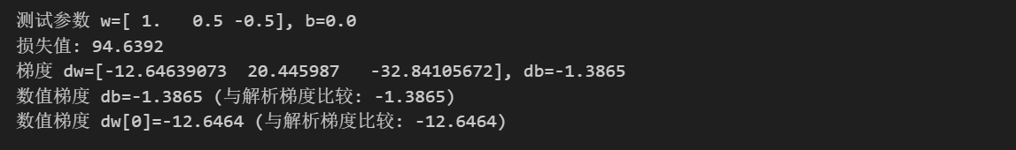
3、实现小批量梯度下降算法
python
def mini_batch_gradient_descent(X, y, w_init=None, b_init=0.0, learning_rate=0.01,
batch_size=32, num_epochs=100, tolerance=1e-6):
"""
小批量梯度下降算法实现
参数:
X: 特征矩阵 (m, n_features)
y: 目标向量 (m,)
w_init: 初始权重向量 (n_features,),如果为None则随机初始化
b_init: 初始偏置标量
learning_rate: 学习率
batch_size: 小批量大小
num_epochs: 最大训练轮数
tolerance: 收敛阈值
返回:
w_history: 权重历史列表
b_history: 偏置历史列表
loss_history: 损失历史列表
"""
m, n_features = X.shape
# 初始化参数
if w_init is None:
w = np.random.randn(n_features) * 0.1
else:
w = w_init.copy()
b = b_init
w_history = [w.copy()]
b_history = [b]
loss_history = [compute_loss(w, b, X, y)]
for epoch in range(num_epochs):
# 打乱数据
indices = np.random.permutation(m)
X_shuffled = X[indices]
y_shuffled = y[indices]
# 分批处理
for start_idx in range(0, m, batch_size):
end_idx = min(start_idx + batch_size, m)
X_batch = X_shuffled[start_idx:end_idx]
y_batch = y_shuffled[start_idx:end_idx]
# 计算小批量梯度
dw, db = compute_batch_gradients(w, b, X_batch, y_batch)
# 更新参数
w -= learning_rate * dw
b -= learning_rate * db
# 计算当前epoch的损失
current_loss = compute_loss(w, b, X, y)
loss_history.append(current_loss)
w_history.append(w.copy())
b_history.append(b)
# 检查收敛
if abs(loss_history[-1] - loss_history[-2]) < tolerance:
print(f"算法在第{epoch+1}轮收敛")
break
# 每10轮打印一次信息
if (epoch + 1) % 10 == 0:
print(f"Epoch {epoch+1}: loss={current_loss:.6f}")
return w_history, b_history, loss_history
# 运行小批量梯度下降
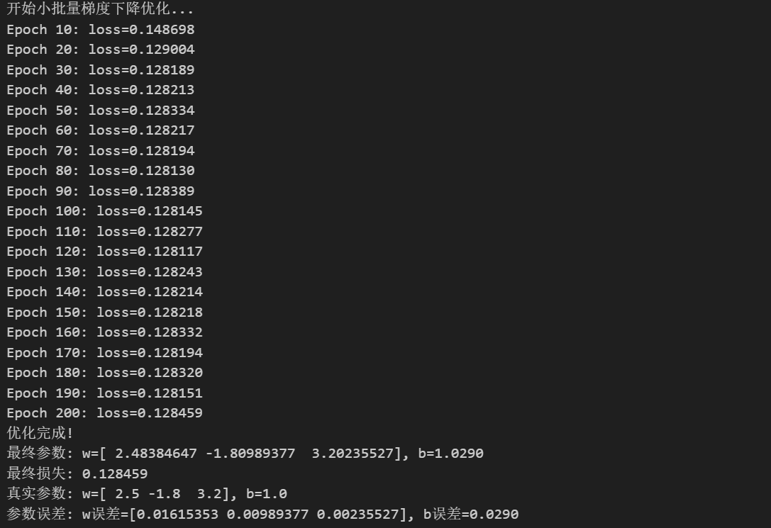
print("开始小批量梯度下降优化...")
w_history, b_history, loss_history = mini_batch_gradient_descent(
X, y,
w_init=np.zeros(n_features),
b_init=0.0,
learning_rate=0.01,
batch_size=32,
num_epochs=200
)
print("优化完成!")
print(f"最终参数: w={w_history[-1]}, b={b_history[-1]:.4f}")
print(f"最终损失: {loss_history[-1]:.6f}")
print(f"真实参数: w={true_w}, b={true_b}")
print(f"参数误差: w误差={np.abs(w_history[-1] - true_w)}, b误差={abs(b_history[-1] - true_b):.4f}")核心就在于batch_size的选择,每轮更新中,从总体样本中随机选出batch_size大小的样本进行更新。
4、可视化学习过程
python
# 可视化损失函数收敛过程
plt.figure(figsize=(12, 5))
plt.subplot(1, 2, 1)
plt.plot(loss_history, 'b-', linewidth=2)
plt.xlabel('训练轮数')
plt.ylabel('损失值')
plt.title('损失函数收敛过程')
plt.grid(True, alpha=0.3)
plt.yscale('log') # 使用对数尺度更好地显示收敛
plt.subplot(1, 2, 2)
plt.plot(loss_history[:50], 'r-', linewidth=2) # 只显示前50轮
plt.xlabel('训练轮数')
plt.ylabel('损失值')
plt.title('损失函数收敛过程 (前50轮)')
plt.grid(True, alpha=0.3)
plt.tight_layout()
plt.show()
print(f"初始损失: {loss_history[0]:.6f}")
print(f"最终损失: {loss_history[-1]:.6f}")
print(f"损失减少: {loss_history[0] - loss_history[-1]:.6f} ({((loss_history[0] - loss_history[-1])/loss_history[0]*100):.1f}%)")
# 可视化参数更新过程
plt.figure(figsize=(15, 5))
for i in range(n_features):
plt.subplot(1, n_features+1, i+1)
w_values = [w[i] for w in w_history]
plt.plot(w_values, linewidth=2, label=f'w{i+1}')
plt.axhline(y=true_w[i], color='r', linestyle='--', alpha=0.7, label=f'真实w{i+1}={true_w[i]}')
plt.xlabel('训练轮数')
plt.ylabel(f'w{i+1}')
plt.title(f'权重 w{i+1} 更新过程')
plt.legend()
plt.grid(True, alpha=0.3)
plt.subplot(1, n_features+1, n_features+1)
plt.plot(b_history, 'orange', linewidth=2, label='b')
plt.axhline(y=true_b, color='r', linestyle='--', alpha=0.7, label=f'真实b={true_b}')
plt.xlabel('训练轮数')
plt.ylabel('偏置 b')
plt.title('偏置参数更新过程')
plt.legend()
plt.grid(True, alpha=0.3)
plt.tight_layout()
plt.show()
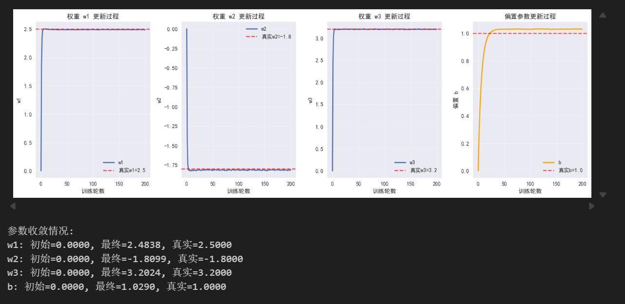
print(f"参数收敛情况:")
for i in range(n_features):
print(f"w{i+1}: 初始={w_history[0][i]:.4f}, 最终={w_history[-1][i]:.4f}, 真实={true_w[i]:.4f}")
print(f"b: 初始={b_history[0]:.4f}, 最终={b_history[-1]:.4f}, 真实={true_b:.4f}")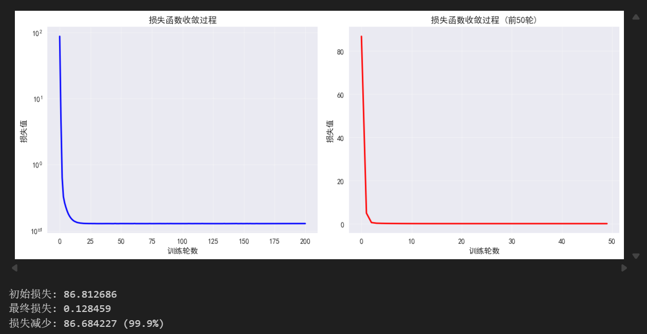
5、误差分析
python
# 预测结果分析
y_pred_final = X @ w_history[-1] + b_history[-1]

plt.figure(figsize=(12, 5))

plt.subplot(1, 2, 1)
plt.scatter(y, y_pred_final, alpha=0.6, color='blue')
plt.plot([y.min(), y.max()], [y.min(), y.max()], 'r--', linewidth=2, label='完美预测线')
plt.xlabel('真实值')
plt.ylabel('预测值')
plt.title('预测结果 vs 真实值')
plt.legend()
plt.grid(True, alpha=0.3)

plt.subplot(1, 2, 2)
residuals = y - y_pred_final
plt.hist(residuals, bins=30, alpha=0.7, color='green')
plt.xlabel('残差')
plt.ylabel('频次')
plt.title('残差分布')
plt.grid(True, alpha=0.3)

plt.tight_layout()
plt.show()

# 计算R²分数
ss_res = np.sum((y - y_pred_final)**2)
ss_tot = np.sum((y - np.mean(y))**2)
r2_score = 1 - (ss_res / ss_tot)

print(f"模型性能分析:")
print(f"R² 分数: {r2_score:.4f}")
print(f"均方根误差 (RMSE): {np.sqrt(np.mean((y - y_pred_final)**2)):.4f}")
print(f"平均绝对误差 (MAE): {np.mean(np.abs(y - y_pred_final)):.4f}")

# 参数收敛分析
print(f"\n参数学习情况:")
for i in range(n_features):
    error = abs(w_history[-1][i] - true_w[i])
    print(f"w{i+1}: 学习到 {w_history[-1][i]:.4f}, 真实值 {true_w[i]:.4f}, 误差 {error:.4f}")
error_b = abs(b_history[-1] - true_b)
print(f"b: 学习到 {b_history[-1]:.4f}, 真实值 {true_b:.4f}, 误差 {error_b:.4f}")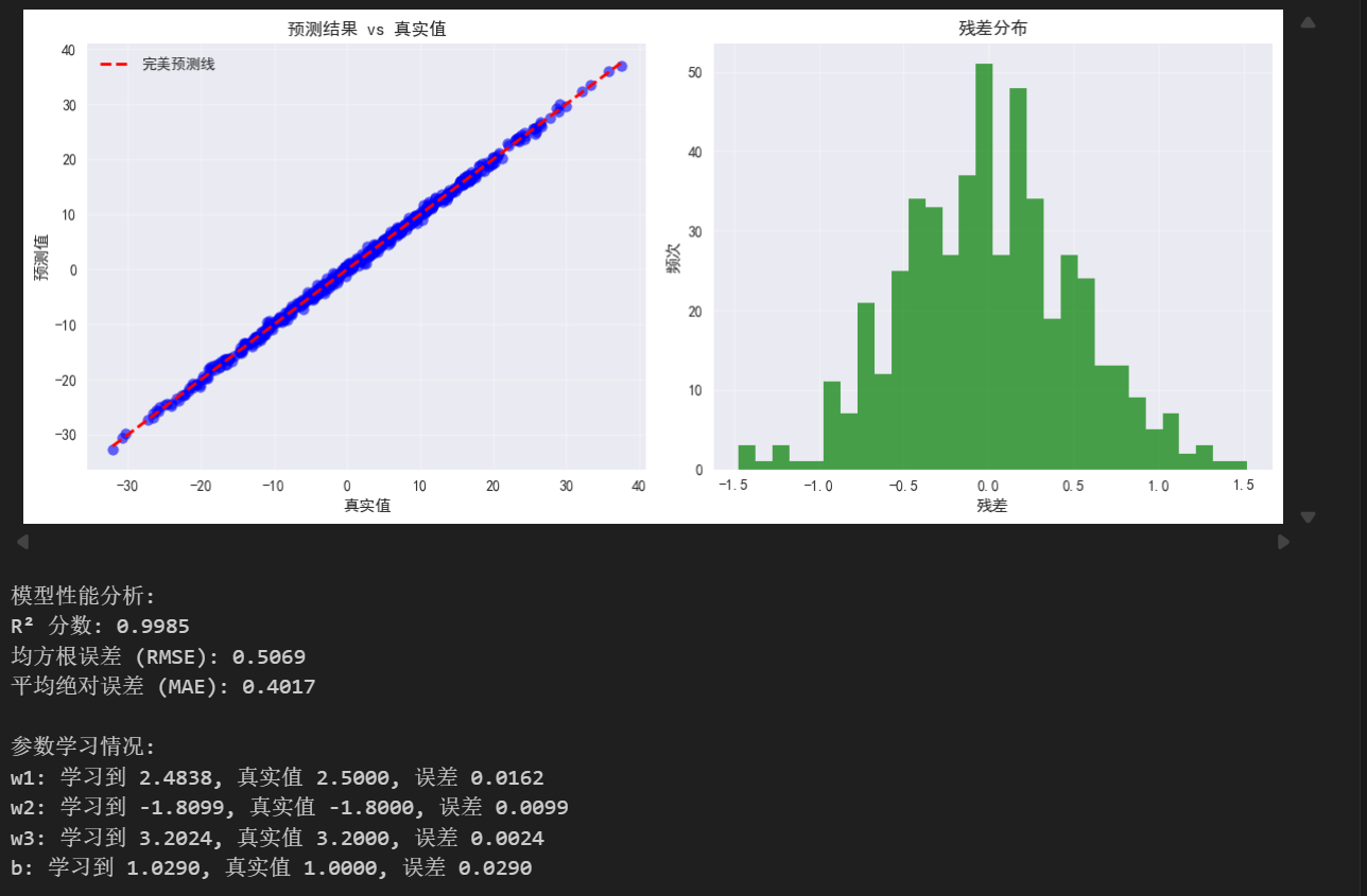
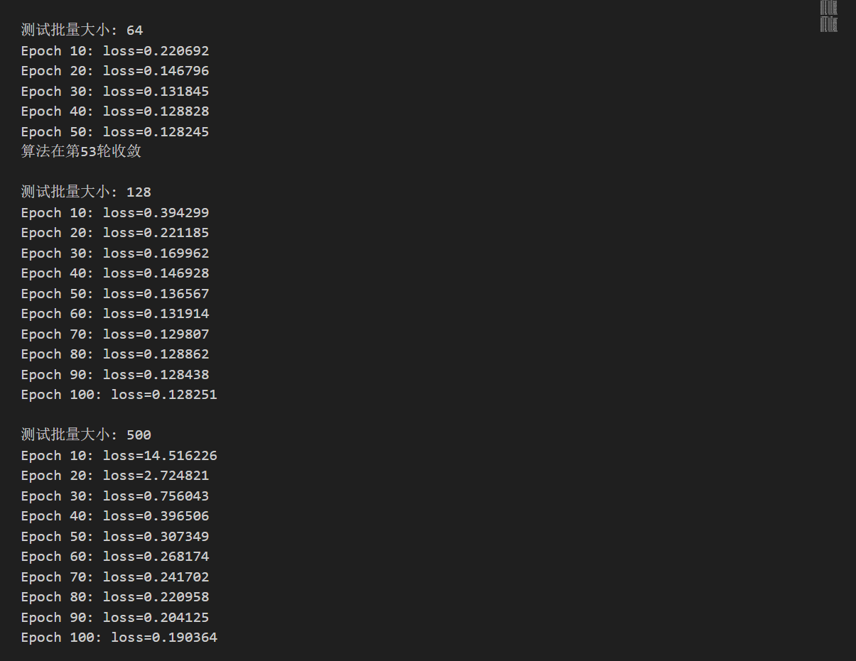
实验不同批量大小对实验结果的影响
python
# 实验不同批量大小
batch_sizes = [1, 16, 32, 64, 128, m]  # m是全批量
results_batch = {}

plt.figure(figsize=(15, 10))

for i, batch_size in enumerate(batch_sizes):
    print(f"\n测试批量大小: {batch_size}")

    # 运行小批量梯度下降
    w_hist, b_hist, loss_hist = mini_batch_gradient_descent(
        X, y, w_init=np.zeros(n_features), b_init=0.0,
        learning_rate=0.01, batch_size=batch_size, num_epochs=100
    )

    results_batch[batch_size] = {
        'w_final': w_hist[-1],
        'b_final': b_hist[-1],
        'loss_final': loss_hist[-1],
        'epochs': len(loss_hist) - 1
    }

    # 绘制损失收敛曲线
    plt.subplot(2, 3, i+1)
    plt.plot(loss_hist, linewidth=2, label=f'batch_size={batch_size}')
    plt.xlabel('训练轮数')
    plt.ylabel('损失值')
    plt.title(f'批量大小 {batch_size} 的收敛')
    plt.grid(True, alpha=0.3)
    plt.legend()

    if len(loss_hist) > 20:
        plt.yscale('log')

plt.tight_layout()
plt.show()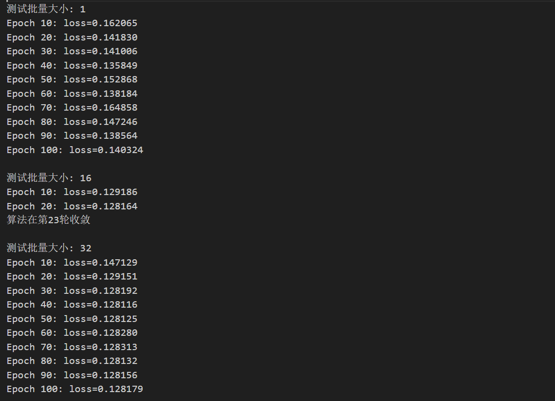
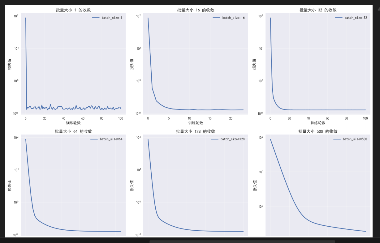
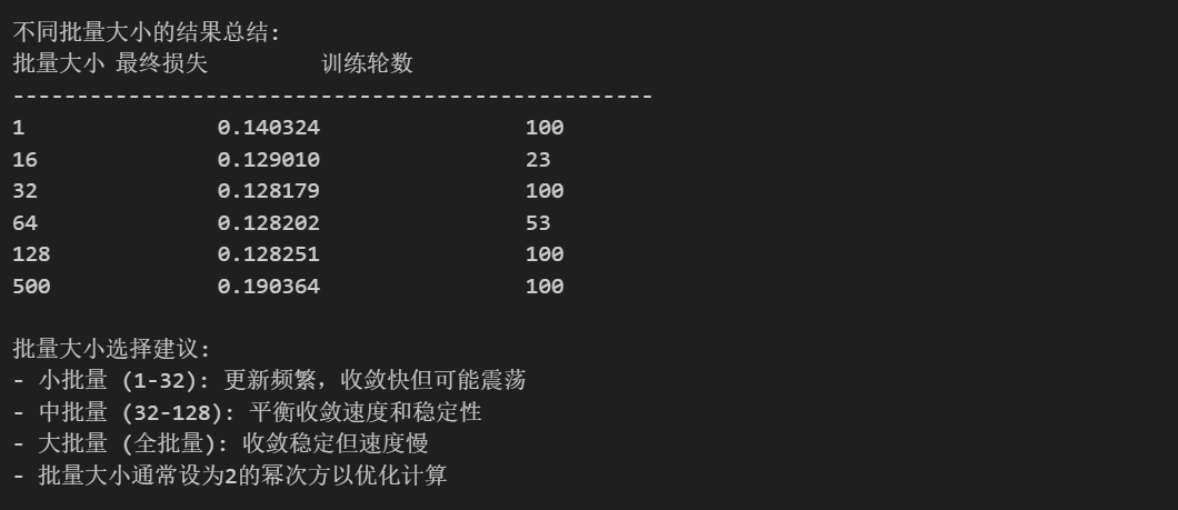
与学习率相似,批量大小的选择也是至关重要的,如果过小会退化为随机梯度下降,过大会退化为全批量梯度下降。总结一个表格来说明如何选择
| 场景 | 推荐批量 | 原因 |
|---|---|---|
| 新手入门 / 线性回归 / 小数据集 | 8 / 16 / 32 | 稳、简单、不震荡 |
| 普通深度学习(分类 / 回归) | 32 / 64 | 平衡速度 + 稳定性 |
| 图像 / CNN/NLP 大模型 | 64 / 128 | GPU 并行效率高 |
| 显存很小(比如笔记本 GPU) | 8 / 16 | 防止显存溢出 |
| 想减少震荡、更平稳 | 64 / 128 | 梯度更准,波动小 |
| 想跳出局部最优、泛化更好 | 16 / 32 | 带一点噪声,更灵活 |
当然,这个批量并不绝对,批量大小是很依赖硬件的,具体到调试上可以参考如下步骤:
- 先设 32,跑一遍
- 不爆显存 → 试 64
- 64 还不爆 → 试 128
- 看曲线:
- 震荡太大 → 调大 batch
- 收敛太慢 / 卡住 → 调小 batch
随机梯度下降为什么会震荡
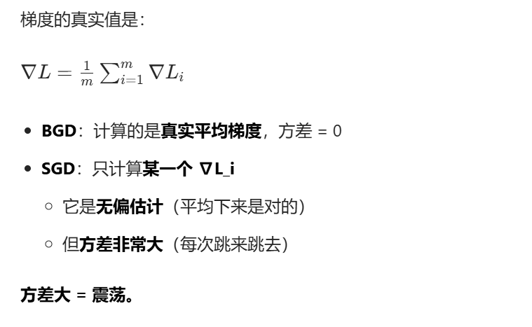
以下山做个比喻:批量梯度下降(BGD)问全班同学 "下山往哪走",取大家的平均方向 → 稳稳下山。 而随机梯度下降(SGD)随机抓一个同学问路,他说东你就东;下一把抓另一个,他说西你就西; 所以你东一下西一下,晃着下山。
当然值得说明的是,震荡虽然看起来乱,但有巨大优点:
- 不容易陷入局部最小值
- 容易跳出鞍点
- 训练速度远快于 BGD
通过这两篇文章的内容,我们已经掌握了深度学习最核心的参数更新方法 ------ 梯度下降。它与反向传播一起,构成了多层感知机(MLP)的训练核心 。而我们前面讲的多元线性回归,正是 MLP 的一个极简特例:它是最简单的线性模型,没有隐藏层、也没有非线性变换。
想要让深度网络真正学会规律,还离不开反向传播。它是基于链式法则的梯度计算算法:从输出层的损失出发,反向逐层计算每一个权重的梯度,再配合梯度下降完成参数更新。正是反向传播,解决了多层神经网络该如何训练的核心难题。
深度学习的标准训练流程可以概括为四步:前向传播(计算预测值)→ 计算损失 → 反向传播(计算梯度)→ 梯度下降(更新参数)
下一篇文章我们会继续讨论反向传播