本篇技术博文摘要 🌟
- 文章始于上节回顾 与概念引入 ,明确了图像分类任务的定义并阐述了选择TensorFlow及CNN作为技术栈的原因。随后,指南详细阐述了环境准备步骤,包括必要库的安装与验证,确保开发环境就绪。
- 在数据集准备 部分,讲解了如何加载标准数据集(如CIFAR-10/MNIST)并进行关键的预处理操作。核心的模型构建章节深入剖析了卷积神经网络(CNN)的架构设计,并提供了模型结构可视化的方法。
- 训练模型部分则完整展示了从编译模型(配置优化器、损失函数与评估指标)、启动训练到实时监控训练过程(如损失与准确率曲线)的完整流程。
- 完成训练后,文章引导读者对模型进行评估与预测,以检验其泛化能力。
- 此外,文章提供了完整的项目代码汇总 、旨在提升模型性能 的实用技巧(如数据增强、超参数调优),并专门设置了常见问题解答环节,针对"CNN的选择"、"Epoch数量的确定"及"内存不足错误处理"等实际开发中典型难题给出解决方案,使本指南不仅具备系统性,更富有实践指导性。
引言 📘
- 在这个变幻莫测、快速发展的技术时代,与时俱进是每个IT工程师的必修课。
- 我是盛透侧视攻城狮,一个"什么都会一丢丢"的网络安全工程师,目前正全力转向AI大模型安全开发新战场。作为活跃于各大技术社区的探索者与布道者,期待与大家交流碰撞,一起应对智能时代的安全挑战和机遇潮流。

上节回顾
目录
[本篇技术博文摘要 🌟](#本篇技术博文摘要 🌟)
[引言 📘](#引言 📘)
[1.TensorFlow 实例 - 图像分类项目](#1.TensorFlow 实例 - 图像分类项目)

1.TensorFlow 实例 - 图像分类项目
- 图像分类是计算机视觉中最基础也最重要的任务之一。
- 本项目将使用 TensorFlow 框架构建一个能够识别不同类别图像的深度学习模型。

1.1什么是图像分类
图像分类是指让计算机自动识别图像中主要物体所属类别的技术。例如:
- 识别照片中是猫还是狗
- 区分不同种类的花朵
- 判断医学影像中的病变类型

1.2技术选型
技术栈如下所示:
- TensorFlow:Google 开发的主流深度学习框架
- Keras:TensorFlow 的高级API,简化模型构建
- Matplotlib:用于可视化训练过程和结果

2.环境准备
2.1安装必要库
bash
pip install tensorflow matplotlib numpy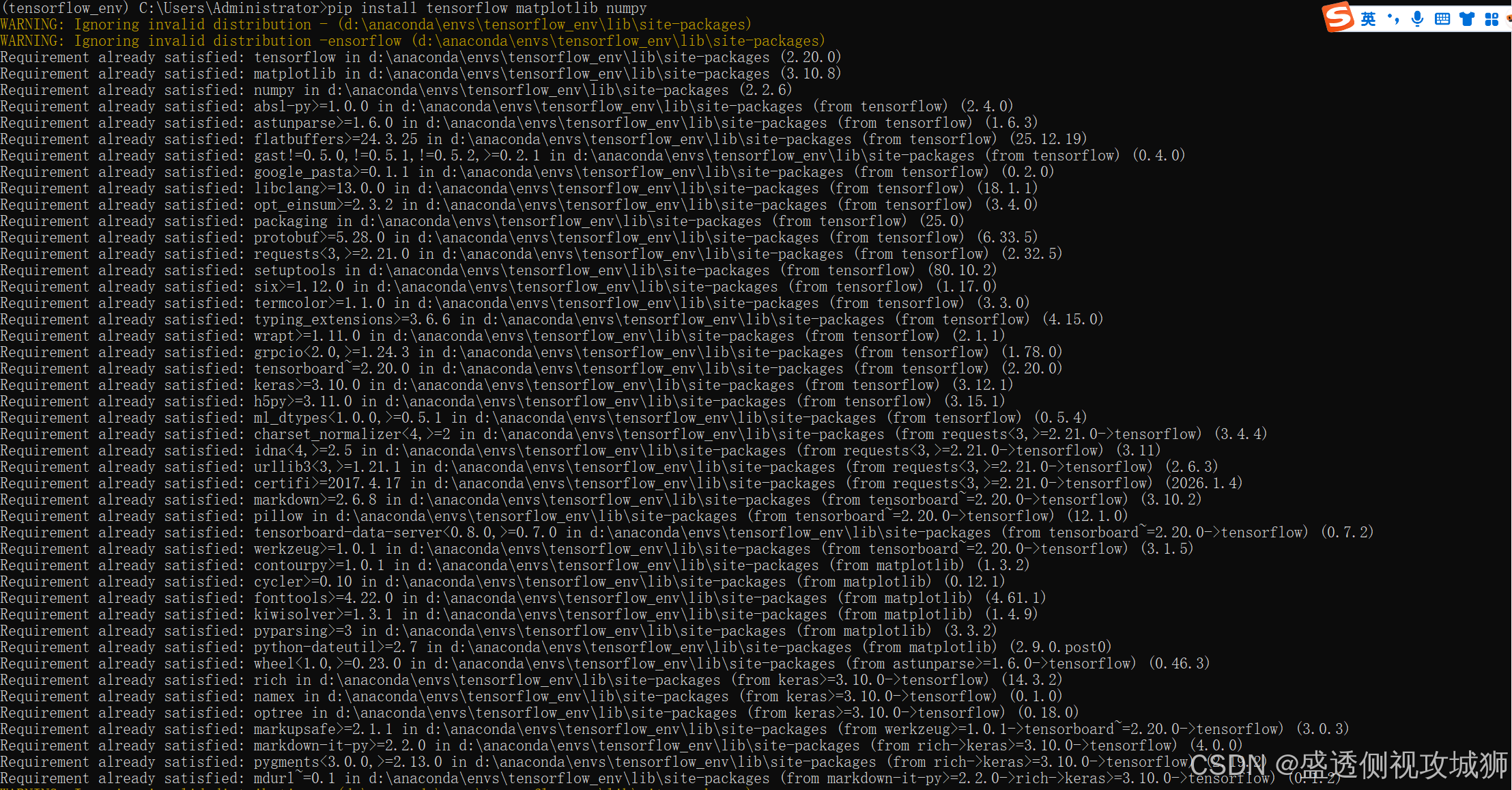
2.2验证安装
python
import tensorflow as tf
print(f"TensorFlow 版本: {tf.__version__}")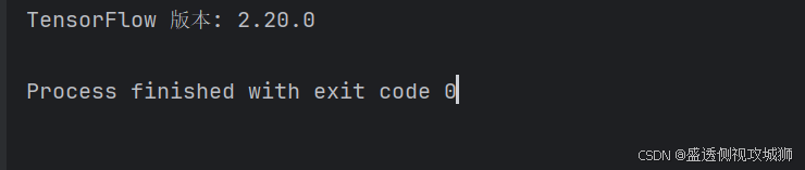

3.数据集准备
- 我们将使用经典的 CIFAR-10 数据集,它包含10个类别的6万张32x32彩色图像
3.1加载数据集
python
from tensorflow.keras.datasets import cifar10

# 加载数据
(train_images, train_labels), (test_images, test_labels) = cifar10.load_data()

# 类别名称
class_names = ['飞机', '汽车', '鸟', '猫', '鹿',
               '狗', '青蛙', '马', '船', '卡车']
3.2数据预处理
python
# 归一化像素值到0-1范围
train_images = train_images / 255.0
test_images = test_images / 255.0

# 查看数据形状
print("训练集图像形状:", train_images.shape)
print("训练集标签形状:", train_labels.shape)
4.构建模型
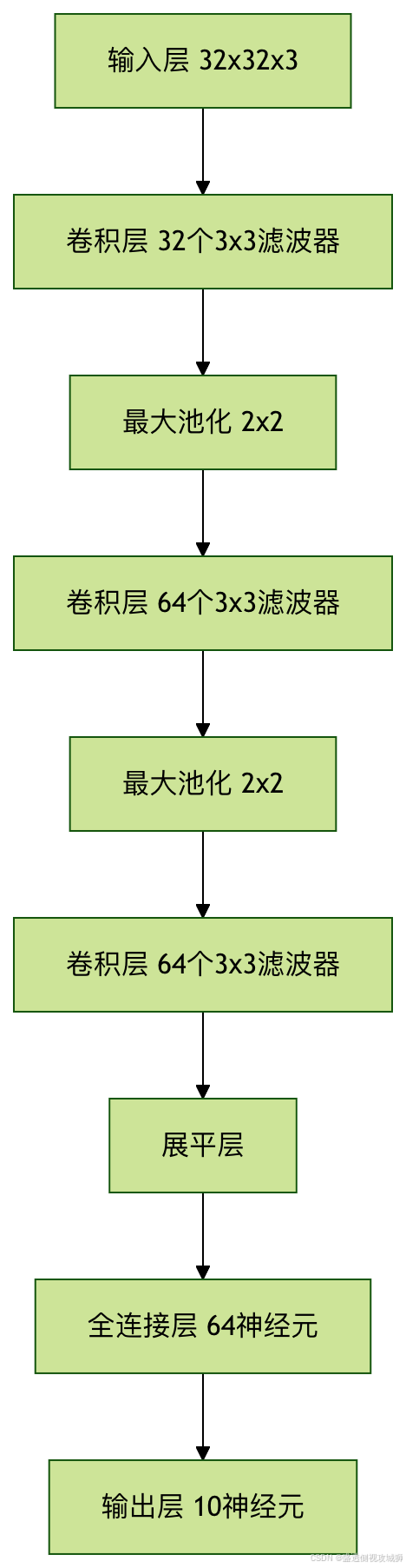
4.1模型架构
- 构建一个卷积神经网络(CNN),这是处理图像任务的经典结构
python
from tensorflow.keras import layers, models

model = models.Sequential([
    # 卷积层1
    layers.Conv2D(32, (3, 3), activation='relu', input_shape=(32, 32, 3)),
    layers.MaxPooling2D((2, 2)),

    # 卷积层2
    layers.Conv2D(64, (3, 3), activation='relu'),
    layers.MaxPooling2D((2, 2)),

    # 卷积层3
    layers.Conv2D(64, (3, 3), activation='relu'),

    # 全连接层
    layers.Flatten(),
    layers.Dense(64, activation='relu'),
    layers.Dense(10)  # 输出层,10个类别
])
4.2模型结构可视化

5.训练模型
5.1编译模型
python
model.compile(optimizer='adam',
              loss=tf.keras.losses.SparseCategoricalCrossentropy(from_logits=True),
              metrics=['accuracy'])
5.2开始训练
python
history = model.fit(train_images, train_labels, epochs=10,
                    validation_data=(test_images, test_labels))
5.3训练过程可视化
python
import matplotlib.pyplot as plt

plt.plot(history.history['accuracy'], label='训练准确率')
plt.plot(history.history['val_accuracy'], label='验证准确率')
plt.xlabel('Epoch')
plt.ylabel('Accuracy')
plt.ylim([0, 1])
plt.legend(loc='lower right')
plt.show()
6.模型评估与预测
6.1评估测试集性能
python
test_loss, test_acc = model.evaluate(test_images, test_labels, verbose=2)
print(f'\n测试准确率: {test_acc}')
6.2进行预测
python
import numpy as np

# 添加softmax层使输出为概率
probability_model = tf.keras.Sequential([model, layers.Softmax()])

# 对测试集前5张图进行预测
predictions = probability_model.predict(test_images[:5])

# 显示预测结果
for i in range(5):
    predicted_label = np.argmax(predictions[i])
    true_label = test_labels[i][0]
    print(f"预测: {class_names[predicted_label]} | 实际: {class_names[true_label]}")
7.项目代码汇总及扩展建议
7.1代码汇总
python
import tensorflow as tf
from tensorflow.keras.datasets import cifar10
from tensorflow.keras import layers, models
import numpy as np
import matplotlib.pyplot as plt
import seaborn as sns
from sklearn.metrics import confusion_matrix, classification_report
import warnings
warnings.filterwarnings('ignore')
# 设置中文字体和图表样式
plt.rcParams['font.sans-serif'] = ['SimHei']
plt.rcParams['axes.unicode_minus'] = False
plt.style.use('seaborn-v0_8-darkgrid')
# 加载数据
(train_images, train_labels), (test_images, test_labels) = cifar10.load_data()
# 类别名称
class_names = ['飞机', '汽车', '鸟', '猫', '鹿',
'狗', '青蛙', '马', '船', '卡车']
# 归一化像素值到0-1范围
train_images = train_images / 255.0
test_images = test_images / 255.0
# 查看数据形状
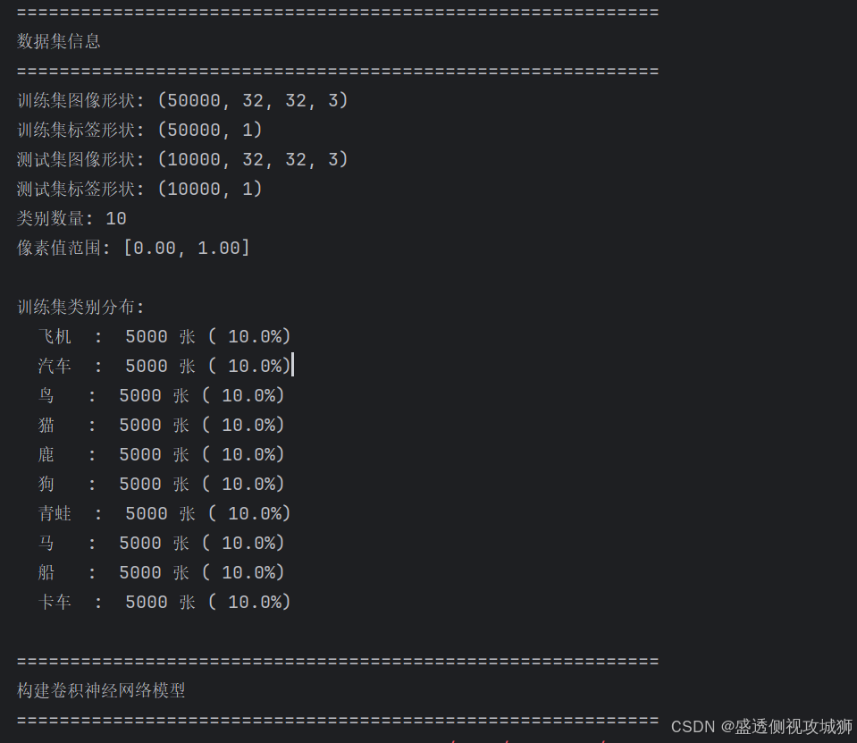
print("=" * 60)
print("数据集信息")
print("=" * 60)
print(f"训练集图像形状: {train_images.shape}")
print(f"训练集标签形状: {train_labels.shape}")
print(f"测试集图像形状: {test_images.shape}")
print(f"测试集标签形状: {test_labels.shape}")
print(f"类别数量: {len(class_names)}")
print(f"像素值范围: [{train_images.min():.2f}, {train_images.max():.2f}]")
# 查看类别分布
print(f"\n训练集类别分布:")
unique, counts = np.unique(train_labels, return_counts=True)
for cls, count in zip(unique, counts):
print(f" {class_names[cls]:<4s}: {count:5d} 张 ({count/len(train_labels)*100:5.1f}%)")
# 可视化部分样本
def visualize_samples(images, labels, num_samples=10):
"""可视化样本图片"""
plt.figure(figsize=(15, 4))
for i in range(num_samples):
plt.subplot(2, 5, i+1)
plt.imshow(images[i])
plt.title(f"{class_names[labels[i][0]]}")
plt.axis('off')
plt.suptitle(f'CIFAR-10 数据集样本 (前{num_samples}张)', fontsize=16, y=1.02)
plt.tight_layout()
plt.show()
# 显示前10个训练样本
visualize_samples(train_images, train_labels, num_samples=10)
# 构建模型
print("\n" + "=" * 60)
print("构建卷积神经网络模型")
print("=" * 60)
model = models.Sequential([
# 卷积层1
layers.Conv2D(32, (3, 3), activation='relu', input_shape=(32, 32, 3)),
layers.MaxPooling2D((2, 2)),
# 卷积层2
layers.Conv2D(64, (3, 3), activation='relu'),
layers.MaxPooling2D((2, 2)),
# 卷积层3
layers.Conv2D(64, (3, 3), activation='relu'),
# 全连接层
layers.Flatten(),
layers.Dense(64, activation='relu'),
layers.Dense(10) # 输出层,10个类别
])
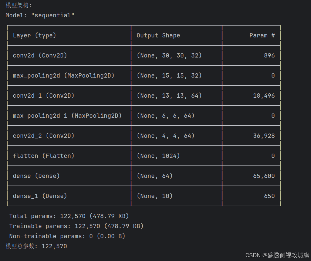
# 显示模型结构
print("模型架构:")
model.summary()
# 计算模型参数总数
total_params = model.count_params()
print(f"模型总参数: {total_params:,}")
# 编译模型
model.compile(optimizer='adam',
loss=tf.keras.losses.SparseCategoricalCrossentropy(from_logits=True),
metrics=['accuracy'])
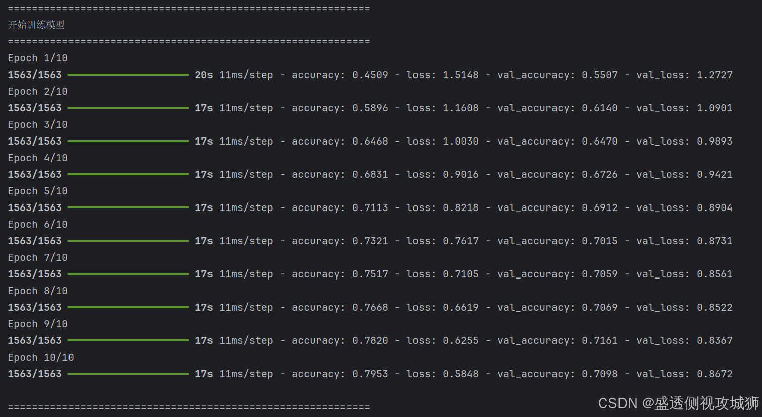
# 训练模型
print("\n" + "=" * 60)
print("开始训练模型")
print("=" * 60)
history = model.fit(train_images, train_labels, epochs=10,
validation_data=(test_images, test_labels),
verbose=1)
# 绘制训练过程中的准确率和损失曲线
def plot_training_history(history):
"""绘制训练历史图表"""
fig, (ax1, ax2) = plt.subplots(1, 2, figsize=(14, 5))
# 准确率曲线
ax1.plot(history.history['accuracy'], 'b-', linewidth=2, label='训练准确率')
ax1.plot(history.history['val_accuracy'], 'r-', linewidth=2, label='验证准确率')
ax1.set_xlabel('Epoch', fontsize=12)
ax1.set_ylabel('准确率', fontsize=12)
ax1.set_title('训练和验证准确率', fontsize=14)
ax1.set_ylim([0, 1])
ax1.legend()
ax1.grid(True, alpha=0.3)
# 损失曲线
ax2.plot(history.history['loss'], 'b-', linewidth=2, label='训练损失')
ax2.plot(history.history['val_loss'], 'r-', linewidth=2, label='验证损失')
ax2.set_xlabel('Epoch', fontsize=12)
ax2.set_ylabel('损失', fontsize=12)
ax2.set_title('训练和验证损失', fontsize=14)
ax2.legend()
ax2.grid(True, alpha=0.3)
plt.suptitle('模型训练历史', fontsize=16, y=1.02)
plt.tight_layout()
plt.show()
# 绘制训练历史
plot_training_history(history)
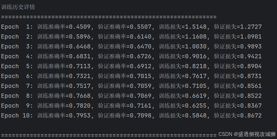
# 输出每个epoch的训练结果
print("\n" + "=" * 60)
print("训练历史详情")
print("=" * 60)
for epoch in range(len(history.history['accuracy'])):
print(f"Epoch {epoch+1:2d}: "
f"训练准确率={history.history['accuracy'][epoch]:.4f}, "
f"验证准确率={history.history['val_accuracy'][epoch]:.4f}, "
f"训练损失={history.history['loss'][epoch]:.4f}, "
f"验证损失={history.history['val_loss'][epoch]:.4f}")
# 评估模型
print("\n" + "=" * 60)
print("模型评估结果")
print("=" * 60)
test_loss, test_acc = model.evaluate(test_images, test_labels, verbose=0)
print(f"测试损失: {test_loss:.4f}")
print(f"测试准确率: {test_acc:.4f}")
# 在测试集上进行预测
print("\n" + "=" * 60)
print("在测试集上进行预测")
print("=" * 60)
# 添加softmax层使输出为概率
probability_model = tf.keras.Sequential([model, layers.Softmax()])
# 对测试集前15张图进行预测
num_test_samples = 15
predictions = probability_model.predict(test_images[:num_test_samples])
# 显示预测结果
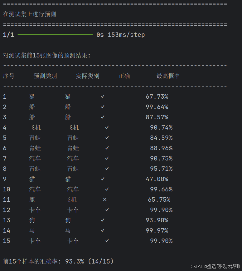
print(f"\n对测试集前{num_test_samples}张图像的预测结果:")
print("-" * 60)
print(f"{'序号':<6} {'预测类别':<8} {'实际类别':<8} {'正确':<8} {'最高概率':<10}")
print("-" * 60)
correct_predictions = 0
for i in range(num_test_samples):
predicted_label = np.argmax(predictions[i])
true_label = test_labels[i][0]
confidence = np.max(predictions[i]) * 100
is_correct = predicted_label == true_label
if is_correct:
correct_predictions += 1
status = "✓" if is_correct else "✗"
print(f"{i+1:<6d} {class_names[predicted_label]:<8} "
f"{class_names[true_label]:<8} {status:<8} {confidence:8.2f}%")
print("-" * 60)
print(f"前{num_test_samples}个样本的准确率: {correct_predictions/num_test_samples*100:.1f}% ({correct_predictions}/{num_test_samples})")
# 可视化前15个测试样本的预测结果
def visualize_predictions(images, true_labels, predictions, class_names, num_samples=15):
"""可视化预测结果"""
num_cols = 5
num_rows = (num_samples + num_cols - 1) // num_cols
plt.figure(figsize=(15, 3*num_rows))
for i in range(num_samples):
plt.subplot(num_rows, num_cols, i+1)
plt.imshow(images[i])
predicted_label = np.argmax(predictions[i])
true_label = true_labels[i][0]
confidence = np.max(predictions[i]) * 100
title_color = 'green' if predicted_label == true_label else 'red'
title_text = f"预测: {class_names[predicted_label]}\n实际: {class_names[true_label]}\n置信度: {confidence:.1f}%"
plt.title(title_text, color=title_color, fontsize=10)
plt.axis('off')
plt.suptitle('测试集预测结果可视化 (绿色=正确, 红色=错误)', fontsize=16, y=1.02)
plt.tight_layout()
plt.show()
# 可视化预测结果
visualize_predictions(test_images, test_labels, predictions, class_names, num_samples=15)
# 混淆矩阵和分类报告
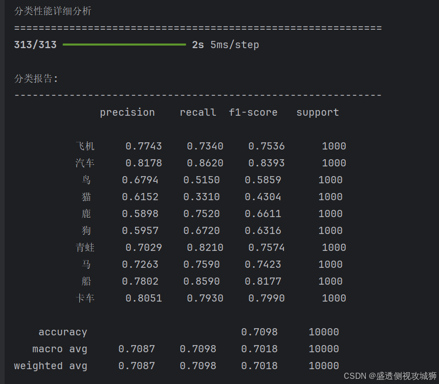
print("\n" + "=" * 60)
print("分类性能详细分析")
print("=" * 60)
# 在完整测试集上进行预测
y_pred_probs = probability_model.predict(test_images)
y_pred = np.argmax(y_pred_probs, axis=1)
y_true = test_labels.flatten()
# 计算混淆矩阵
cm = confusion_matrix(y_true, y_pred)
# 绘制混淆矩阵
plt.figure(figsize=(10, 8))
sns.heatmap(cm, annot=True, fmt='d', cmap='Blues',
xticklabels=class_names, yticklabels=class_names)
plt.xlabel('预测类别', fontsize=12)
plt.ylabel('实际类别', fontsize=12)
plt.title('混淆矩阵', fontsize=16)
plt.tight_layout()
plt.show()
# 输出分类报告
print("\n分类报告:")
print("-" * 60)
print(classification_report(y_true, y_pred, target_names=class_names, digits=4))
# 计算每个类别的准确率
class_accuracies = []
for i in range(len(class_names)):
mask = y_true == i
if np.sum(mask) > 0:
accuracy = np.sum(y_pred[mask] == i) / np.sum(mask) * 100
else:
accuracy = 0
class_accuracies.append(accuracy)
# 可视化每个类别的准确率
plt.figure(figsize=(12, 6))
bars = plt.bar(range(len(class_names)), class_accuracies, color='skyblue')
plt.xlabel('类别', fontsize=12)
plt.ylabel('准确率 (%)', fontsize=12)
plt.title('每个类别的测试准确率', fontsize=16)
plt.xticks(range(len(class_names)), class_names, rotation=45, ha='right')
plt.ylim(0, 100)
plt.grid(axis='y', alpha=0.3)
# 在每个柱子上添加准确率数值
for bar, acc in zip(bars, class_accuracies):
height = bar.get_height()
plt.text(bar.get_x() + bar.get_width()/2., height + 1,
f'{acc:.1f}%', ha='center', va='bottom', fontsize=10)
plt.tight_layout()
plt.show()
# 保存模型
try:
model.save('cifar10_cnn_model.h5')
print("\n模型已保存为 'cifar10_cnn_model.h5'")
except:
print("\n模型保存失败")
print("\n" + "=" * 60)
print("代码执行完成!")
print("=" * 60)7.2提高模型性能的方法
- 增加网络深度(更多卷积层)
- 使用数据增强技术
- 尝试不同的优化器和学习率
- 添加批归一化层
7.3实际应用方向
- 医学影像分析
- 自动驾驶中的物体识别
- 工业质检系统
- 安防监控系统

8.常见问题解答
8.1为什么选择CNN而不是普通神经网络
- CNN通过局部连接和权值共享能更好地捕捉图像的空间特征,且参数更少
8.2如何选择合适的epoch数量
- 观察验证集准确率,当不再提升时停止训练,避免过拟合
8.3遇到内存不足错误怎么办
- 可以减小batch size,或使用更小的图像尺寸
欢迎各位彦祖与热巴畅游本人专栏与技术博客
你的三连是我最大的动力
点击➡️指向的专栏名即可闪现
➡️计算机组成原理****
➡️操作系统
➡️****渗透终极之红队攻击行动********
➡️ 动画可视化数据结构与算法
➡️ 永恒之心蓝队联纵合横防御
➡️****华为高级网络工程师********
➡️****华为高级防火墙防御集成部署********
➡️ 未授权访问漏洞横向渗透利用
➡️****逆向软件破解工程********
➡️****MYSQL REDIS 进阶实操********
➡️****红帽高级工程师
➡️红帽系统管理员********
➡️****HVV 全国各地面试题汇总********