INT303 Coursework2 贷款批准预测模型（对整个大数据知识的应用）

文章目录

• [1. 环境配置](#1. 环境配置)
• • [1.1 Anaconda 设置](#1.1 Anaconda 设置)
  • [1.2 使用的包](#1.2 使用的包)
• [2. 作业概要](#2. 作业概要)
• [3. 数据概览/尝试分析](#3. 数据概览/尝试分析)
• • [3.1 加载数据集](#3.1 加载数据集)
  • [3.2 展示数据](#3.2 展示数据)
  • [3.3 数据信息和统计](#3.3 数据信息和统计)
  • [3.4 确定缺失值](#3.4 确定缺失值)
  • [3.5 确定重复值](#3.5 确定重复值)
• [4. 探索性数据分析以及可视化](#4. 探索性数据分析以及可视化)
• • [4.1 数据分布](#4.1 数据分布)
  • [4.2 特征关系](#4.2 特征关系)
• [5. 数据预处理](#5. 数据预处理)
• • [5.1 处理缺失值](#5.1 处理缺失值)
  • [5.2 类别型特征编码](#5.2 类别型特征编码)
• [6. 特征工程](#6. 特征工程)
• • [5.3 数据标准化](#5.3 数据标准化)
  • [5.4 训练集和测试集的划分](#5.4 训练集和测试集的划分)
• [7. 模型选择和训练](#7. 模型选择和训练)
• • [7.1 初始化以及训练模型](#7.1 初始化以及训练模型)
• [8. 模型评估](#8. 模型评估)
• • 8.1评估过程
• [8.2 评估比较](#8.2 评估比较)
• [9. 总结](#9. 总结)

1. 环境配置

1.1 Anaconda 设置

关于使用 Anaconda 的相关设置在上次的 Coursework1 中已经提及 Coursework1讲解。

想了解更多 Anaconda 相关设置也可以参考这篇对于 Anaconda 相关问题讲解的文章 Anaconda 讲解。

1.2 使用的包

这次作业我使用的包如下，但有的包不是必须的，而且你也可以加一些额外想要的内容，因此仅作参考。

pandas、numpy、matplotlib、seaborn、sklearn、kagglehub。

2. 作业概要

这次作业要求是通过一个贷款批准预测模型来检验我们下半学期学习的知识。这次作业中老师不仅给出了每步操作需要做什么还具体给出了提示，因此难度不是很高，但是需要我们做的操作比较多。

我为了让整个过程更加合理，又能提现各个打分项因此对于原来的任务排版做了重新排版。后面我会将每一个任务和整个环节都标注清楚。

比如这里老师给出的文件已经完成了大部分环境的导入，以及我们要分析的数据也保存到了我们的电脑上的C:\Users<你的用户名>.cache\kagglehub\datasets\architsharma01\loan-approval-prediction-dataset\versions<版本号>文件夹下（所以这里并不是我们当前工程的文件夹 下，这一点确实比较麻烦），相关的代码如下。

import pandas as pd
import numpy as np
import matplotlib.pyplot as plt
import seaborn as sns

from sklearn.model_selection import train_test_split, GridSearchCV
from sklearn.preprocessing import LabelEncoder, StandardScaler
from sklearn.impute import SimpleImputer
from sklearn.metrics import accuracy_score, f1_score, roc_auc_score, confusion_matrix, classification_report, roc_curve
from sklearn.linear_model import LogisticRegression
from sklearn.ensemble import RandomForestClassifier, GradientBoostingClassifier

# Optional for interpretation
#import shap


import kagglehub
import pandas as pd
path = kagglehub.dataset_download("architsharma01/loan-approval-prediction-dataset")
file_path = path + "/loan_approval_dataset.csv"
df= pd.read_csv(file_path)

比如这里pandas导入了两遍，这些都是不完美的地方。但是鉴于这是老师给的，所以就不修改了吧。

我们可以先打开这个数据集文件先看看。

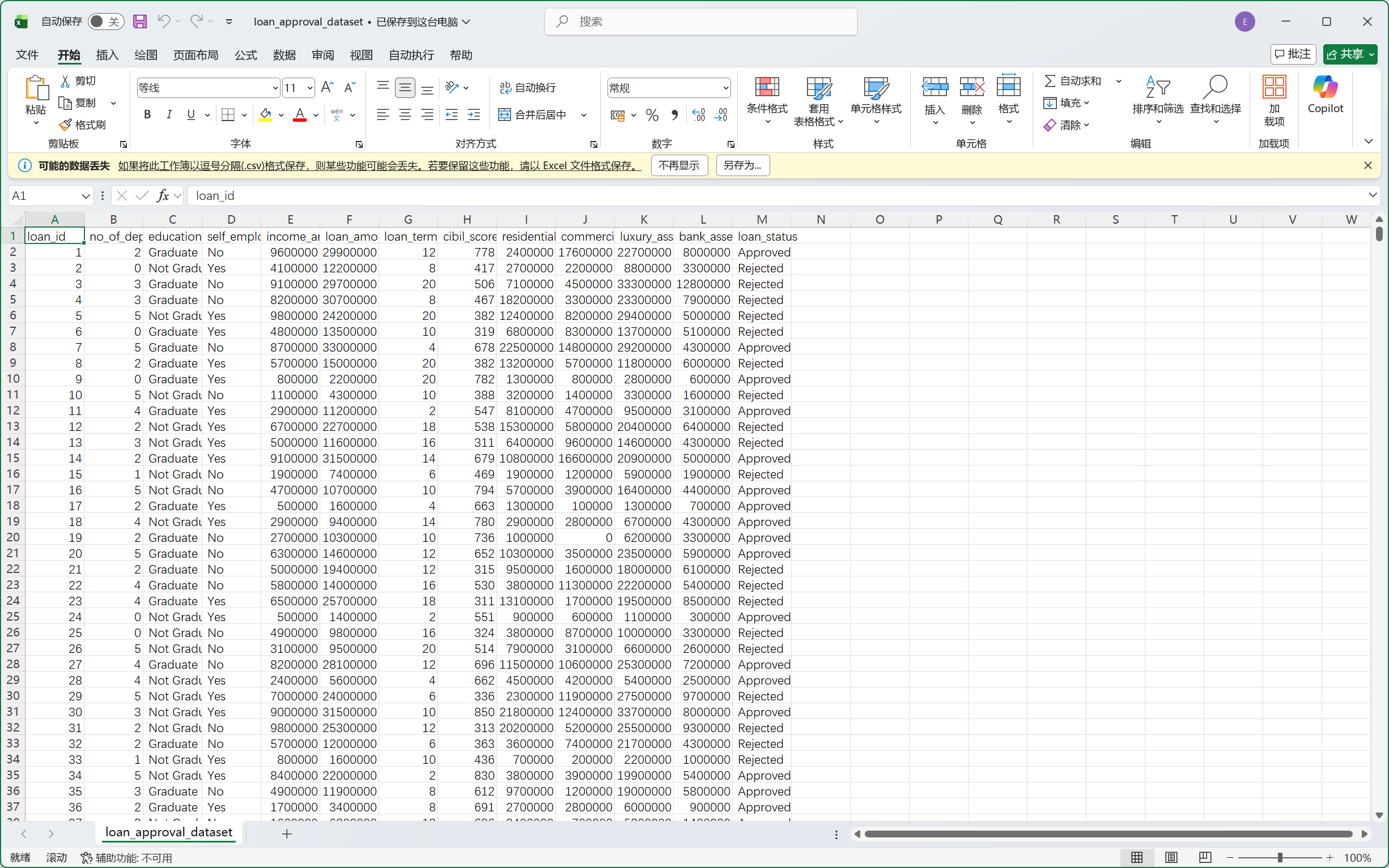
我们可以稍微对这里的数据有些初步认识，但是这里并不清晰，我们可以通过下一个环节来对数据有个清晰的基础认识。

3. 数据概览/尝试分析

我们拿到数据的时候可以先进行操作以对数据有个大致的认识。比如我们可以看看是否有缺失值是否有错误值等等。

3.1 加载数据集

任务1.1要求我们先加载数据集，这一步很简单。

# Task 1.1: Load the dataset
# Assuming 'loan_prediction.csv' is in the current directory
df= pd.read_csv(file_path)

3.2 展示数据

然后任务1.2要求我们展示一下前5行数据，这个操作也很简单。

# Task 1.2: Display the first 5 rows
print("First 5 rows of the dataset:")
print(df.head())

输出结果如下。

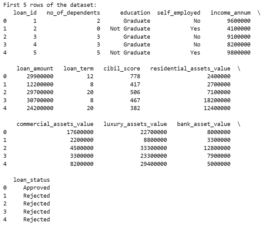
当然我们可以把这个结果跟之前我们看的数据进行对比，我们会发现其是一致的。这个操作其实跟我们刚刚查看文件是一样的，我们通过直接查看数据集从而尝试发现一些规律。

3.3 数据信息和统计

任务1.3要求我们打印数据集信息以及描述性统计。

# Task 1.3: Print info and describe
print("Dataset Info:")
print(df.info())

print("\nDescriptive Statistics:")
print(df.describe())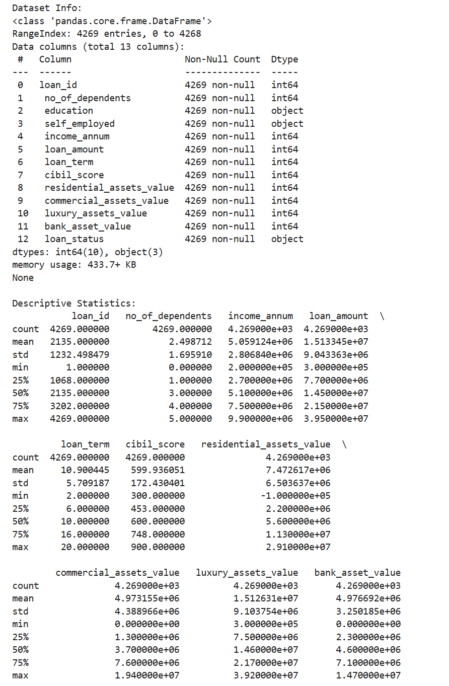

通过这里输出的结果，我们可以清晰看到这里education、self_employed、loan_status都是非数字，因此后续我们对里的数据可能需要处理。我们还可以检查一下非空值，这里刚好和总数一致，说明这里不需要处理缺失的值。其余的值我们可以稍微看看，但似乎也没有什么问题。我们可以进行进一步的操作观察一下。

3.4 确定缺失值

任务1.4让我们详细确认一下是否有缺失值。

# Task 1.4: Identify missing values
print("\nMissing Values per Column:")
print(df.isnull().sum())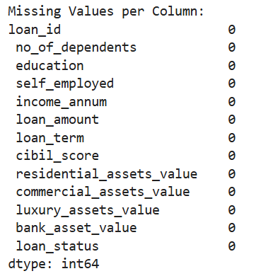

正如我们刚刚通过info观察的一样的确没有，当然这样操作结果会更清晰。

3.5 确定重复值

任务1.5要求我们查看是否有重复的行。

# Task 1.5: Check for duplicate rows
print("\nNumber of duplicate rows:")
print(df.duplicated().sum())

结果也是没有。

这便是一个初步的数据概览，我们后面可以对数据进行可视化从而进行一个进一步的分析。

4. 探索性数据分析以及可视化

这一步是在前面的基础上用可视化来尝试分析数据之间的关系，从而尝试找出判断贷款是否通过与哪些数据有关。

4.1 数据分布

任务4.1让我们用直方图和箱线图来展示数据的分布情况。

我们一共有13列，其中有3列不是数值型数据，剩余的10列中其中有id，这个的分布是没有意义的，我们无需研究对于剩余的9个数据我们都可以做直方图和箱线图去研究数据的分布情况。

我这里建议将这两个图做成两个子图在一张图内，更加高级专业。而这9组数据分成9次展示，这样更加清晰。

因此每组的代码如下。

plt.figure(figsize=(12, 4))
plt.subplot(1,2,1)
sns.histplot(df[' no_of_dependents'], kde=True)
plt.title('no_of_dependents - Histogram')
plt.subplot(1,2,2)
sns.boxplot(y=df[' no_of_dependents'])
plt.title('no_of_dependents - Boxplot')
plt.show()

plt.figure(figsize=(12,4))
plt.subplot(1,2,1)
sns.histplot(df[' income_annum'], kde=True)
plt.title('income_annum - Histogram')
plt.subplot(1,2,2)
sns.boxplot(y=df[' income_annum'])
plt.title('income_annum - Boxplot')
plt.show()

plt.figure(figsize=(12,4))
plt.subplot(1,2,1)
sns.histplot(df[' loan_amount'], kde=True)
plt.title('loan_amount - Histogram')
plt.subplot(1,2,2)
sns.boxplot(y=df[' loan_amount'])
plt.title('loan_amount - Boxplot')
plt.show()

plt.figure(figsize=(12,4))
plt.subplot(1,2,1)
sns.histplot(df[' loan_term'], kde=True)
plt.title('loan_term - Histogram')
plt.subplot(1,2,2)
sns.boxplot(y=df[' loan_term'])
plt.title('loan_term - Boxplot')
plt.show()

plt.figure(figsize=(12,4))
plt.subplot(1,2,1)
sns.histplot(df[' cibil_score'], kde=True)
plt.title('cibil_score - Histogram')
plt.subplot(1,2,2)
sns.boxplot(y=df[' cibil_score'])
plt.title('cibil_score - Boxplot')
plt.show()

plt.figure(figsize=(12,4))
plt.subplot(1,2,1)
sns.histplot(df[' residential_assets_value'], kde=True)
plt.title('residential_assets_value - Histogram')
plt.subplot(1,2,2)
sns.boxplot(y=df[' residential_assets_value'])
plt.title('residential_assets_value - Boxplot')
plt.show()

plt.figure(figsize=(12,4))
plt.subplot(1,2,1)
sns.histplot(df[' commercial_assets_value'], kde=True)
plt.title('commercial_assets_value - Histogram')
plt.subplot(1,2,2)
sns.boxplot(y=df[' commercial_assets_value'])
plt.title('commercial_assets_value - Boxplot')
plt.show()

plt.figure(figsize=(12,4))
plt.subplot(1,2,1)
sns.histplot(df[' luxury_assets_value'], kde=True)
plt.title('luxury_assets_value - Histogram')
plt.subplot(1,2,2)
sns.boxplot(y=df[' luxury_assets_value'])
plt.title('luxury_assets_value - Boxplot')
plt.show()

plt.figure(figsize=(12,4))
plt.subplot(1,2,1)
sns.histplot(df[' bank_asset_value'], kde=True)
plt.title('bank_asset_value - Histogram')
plt.subplot(1,2,2)
sns.boxplot(y=df[' bank_asset_value'])
plt.title('bank_asset_value - Boxplot')
plt.show()

我们刚刚提到有些数据并非数值型，这些数据只是不能做成箱线图，但是还是可以做成直方图。

对应的代码如下。

plt.figure(figsize=(6,4))
sns.countplot(x=' education', data=df)
plt.title('education - Bar Plot')
plt.show()

plt.figure(figsize=(6,4))
sns.countplot(x=' self_employed', data=df)
plt.title('self_employed - Bar Plot')
plt.show()

plt.figure(figsize=(6,4))
sns.countplot(x=' loan_status', data=df)
plt.title('loan_status - Bar Plot')
plt.show()

我们这一环节是用直方图和箱线图来展示数据的分布情况，因此我们无法直接得到我们想要得到的贷款是否通过与哪些数据有关这样的直接联系，我们只能得到一些数据分布情况的信息。

比如我们这次数据都相对比较平衡，而且我们的样本量很大，所以我们可以得到的结论是这个数据集有一定的代表性，我们在这个数据集上得到的结论可以被认为是可靠的。

当然这里比如'residential_assets_value'和'commercial_assets_value' 的分布并不平均，大部分值集中在数值较小的区间内。

4.2 特征关系

我们现在尝试分析特征之间的关系。

我们依然可以使用箱线图来展示特征之间的关系。

我们这里不需要将所有的特征之间两两排列组合而展示所有特征之间的关系，我们要回到我们这次作业的目的本身。我们想要研究贷款批准情况和这些特征之间的关系从而得到一个贷款批准预测模型。

因此我们需要研究的是这些特征与批准情况的关系，然后我们依然不需要考虑id那一列，因为那一项在研究时候没有实际意义。

所以这次我们应该是11张图，当然还是分开展示，更加清晰，代码如下。

plt.figure(figsize=(6,4))
sns.boxplot(x=' loan_status', y=' no_of_dependents', data=df)
plt.title('no_of_dependents vs Loan Status')
plt.show()

plt.figure(figsize=(6,4))
sns.boxplot(x=' loan_status', y=' income_annum', data=df)
plt.title('Income vs Loan Status')
plt.show()

plt.figure(figsize=(6,4))
sns.boxplot(x=' loan_status', y=' loan_amount', data=df)
plt.title('Loan Amount vs Loan Status')
plt.show()

plt.figure(figsize=(6,4))
sns.boxplot(x=' loan_status', y=' loan_term', data=df)
plt.title('Loan Term vs Loan Status')
plt.show()

plt.figure(figsize=(6,4))
sns.boxplot(x=' loan_status', y=' cibil_score', data=df)
plt.title('CIBIL Score vs Loan Status')
plt.show()

plt.figure(figsize=(6,4))
sns.boxplot(x=' loan_status', y=' residential_assets_value', data=df)
plt.title('Residential Assets Value vs Loan Status')
plt.show()

plt.figure(figsize=(6,4))
sns.boxplot(x=' loan_status', y=' commercial_assets_value', data=df)
plt.title('Commercial Assets Value vs Loan Status')
plt.show()

plt.figure(figsize=(6,4))
sns.boxplot(x=' loan_status', y=' luxury_assets_value', data=df)
plt.title('Luxury Assets Value vs Loan Status')
plt.show()

plt.figure(figsize=(6,4))
sns.boxplot(x=' loan_status', y=' bank_asset_value', data=df)
plt.title('Bank Assets Value vs Loan Status')
plt.show()

但是我们这里的数据有两个不是数值型的，因此我们不能使用箱线图，但我们可以使用堆叠条形图来展示这种类别型数据之间的关系。

代码如下。

pd.crosstab(df[' education'], df[' loan_status']).plot(kind='bar', stacked=True, figsize=(6,4))
plt.title('Education vs Loan Status')
plt.xlabel('Education')
plt.ylabel('Count')
plt.show()

pd.crosstab(df[' self_employed'], df[' loan_status']).plot(kind='bar', stacked=True, figsize=(6,4))
plt.title('Self Employed vs Loan Status')
plt.xlabel('Self Employed')
plt.ylabel('Count')
plt.show()

展现数据关系还可以使用散点图和热力图，这些也是展现数据之间关系的有用工具。

对于散点图，我们选取两组特征将其变成一个二维散点图，然后使用不同颜色区分批准情况。

如这里我抽取贷款金额和信用分两组数据，因为我认为这两组数据与批准情况有很大关系。

相关代码如下。

plt.figure(figsize=(10, 6))
scatter = sns.scatterplot(x=' cibil_score', y=' loan_amount', 
                          hue=' loan_status', data=df,
                          s=100, alpha=0.7)

plt.title('Credit Score (CIBIL) vs Loan Amount')
plt.xlabel('CIBIL Credit Score')
plt.ylabel('Loan Amount')
plt.show()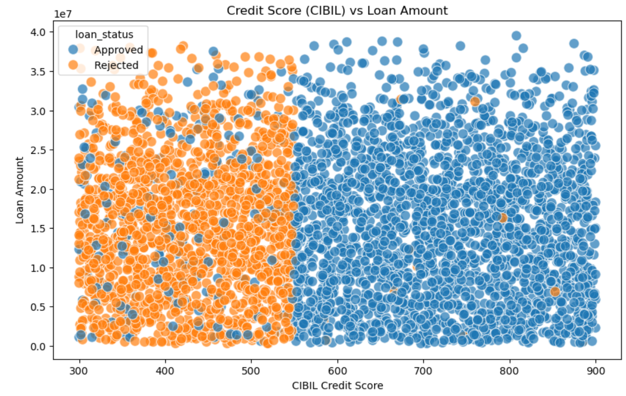

通过这个图我们可以清楚看到信誉分更高的容易获得贷款，其中大概550是个分界线，而右边的蓝色中散落的橙色的点是无规律的，这告诉我们有一些其他因素会决定贷款是否批准，这些是除贷款金额之外的。

我们还可以使用热力图去查看特征之间的关系，这是一种可以获得数据之间关系非常直接的方式。当然只能对数据类型的数据使用。

plt.figure(figsize=(10,8))
# Use numerical features
numerical_df = df.select_dtypes(include='number')
# Drop Loan ID
numerical_df = numerical_df.drop('loan_id', axis=1)
corr = numerical_df.corr()
sns.heatmap(corr, annot=True, cmap='coolwarm')
plt.title('Correlation Heatmap of Numerical Features')
plt.show()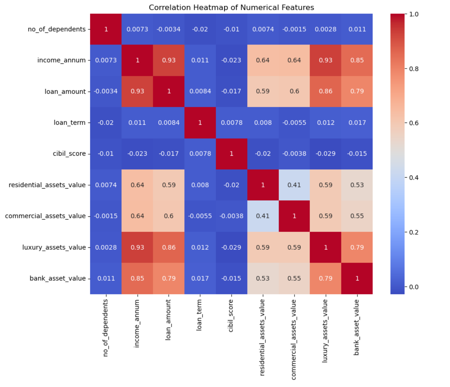

我们可以看出年收入和贷款金额高度相关，而奢侈品资产价值和银行资产价值高度相关。这里CIBIL评分、贷款期限、受扶养人数量与其他特征之间的相关性就较低了。

我们现在总结一下我们获得的发现有哪些：

1. 贷款批准情况与教育以及是否是内部员工无关，因为这两个特征中不同类别有相似的数据模式。
2. CIBIL得分高的贷款通常会获得批准，但得分低的贷款通常不会获得批准。这可能是我们确定贷款批准情况的关键依据。
3. 年收入、贷款金额以及奢侈品资产价值、银行资产价值之间存在高度相关性。CIBIL评分与其他特征之间的相关性通常较低。贷款期限、受抚养人数量与CIBIL评分情况相似。

5. 数据预处理

现在我们要进行数据预处理以方便我们后续训练数据以及预测数据。

我们需要提前复制一份以避免修改原始数据。

# Create a copy to avoid modifying the original DataFrame
df_processed = df.copy()

5.1 处理缺失值

任务3.1要求我们处理缺失值。

一般数据预处理的重点在于缺失值的处理，但是这里我们之前就确定了没有缺失值。

对于一般数据来说我们可以用平均值/中位数来填写数值型数据的缺失值，用众数来填写分类型数据的缺失值。

我们这里出示一个符合上述逻辑的代码，而且会展示最后的缺失值情况。

# Identify all columns with missing values
columns_with_missing = df_processed.columns[df_processed.isnull().any()].tolist()
for column in columns_with_missing:
    missing_count = df_processed[column].isnull().sum()
    # If it is numerical
    if df_processed.select_dtypes(include='number').columns:
        # Select strategy based on data distribution
        skewness = df_processed[column].skew()
        # Use median for skewed distribution
        if abs(skewness) > 0.5:
            fill_value = df_processed[column].median()
        # Use mean for symmetric distribution
        else:
            fill_value = df_processed[column].mean()
    # If it is categorical
    else:
        # Use mode
        # If no mode, it uses Unknown
        fill_value = df_processed[column].mode()[0] if not df_processed[column].mode().empty else 'Unknown'
        df_processed[column].fillna(fill_value, inplace=True)
# Check after imputation
print("Missing values after imputation:")
print(df_processed.isnull().sum())

当然你也可以说这里没有缺失值，所以不需要进行处理。

5.2 类别型特征编码

任务3.2要求我们将类别型数据进行编码，从而将其变为可以处理的数值型数据。

一般这种转换有两种：标签编码（LabelEncoder）和独热编码（OneHotEncoder），前者的缺点是可能会引入虚假的大小关系，后者的缺点是会增加特征维度。

因为这里的'education', 'self_employed', 'loan_status'这三类都是只有两个值，因此无需担心使用独热编码增加太多特征维度。

# Here using the OneHotEncoder to convert categorical columns to numerical
from sklearn.preprocessing import OneHotEncoder

# Columns that require encoding
onehot_columns = [' education', ' self_employed', ' loan_status']
# Create OneHotEncoder
ohe = OneHotEncoder(sparse_output=False, drop='first')
encoded_array = ohe.fit_transform(df_processed[onehot_columns])
# New column name
feature_names = ohe.get_feature_names_out(onehot_columns)
# Create DataFrame
encoded_df = pd.DataFrame(encoded_array, columns=feature_names, index=df_processed.index)
# Delete the original columns
df_processed = df_processed.drop(columns=onehot_columns)
# Add to the original dataset
df_processed = pd.concat([df_processed, encoded_df], axis=1)
# Print the created row name for Task 3.4
print(f"New column created: {list(feature_names)}")

这里的代码还将打印新增加的特征名。

这样我们也可以清晰知道这里的值0和1所代表的具体意思。

6. 特征工程

任务4.1希望我们添加一些新的特征，这一步可能会提升模型的表现。当然我们这样的操作需要一定的合理性，我们不能为了模型的结果而增加新的特征，比如我们直接按照结果作为特征进行输入就是错误的。

这一步操作的启发式思想可以来源于我们前面4.1和4.2节所得到的结论。

我们现在可以创建一个新的特征，这个特征是总资产，它包含住宅资产、商品资产、奢侈品资产、银行资产。这些特征之间本来就相关，我们用一个特征将这些全部涵盖起来，而这在现实过程中也是合理的合并，这样我们就减少了多重共线性。这么做还有一个优点是可以减少特征数，方便我们后续计算。

df_processed[' total_assets'] = (
    df_processed[' residential_assets_value'] +
    df_processed[' commercial_assets_value'] +
    df_processed[' luxury_assets_value'] +
    df_processed[' bank_asset_value']
)
assets_to_drop = [
    ' residential_assets_value',
    ' commercial_assets_value',
    ' luxury_assets_value',
    ' bank_asset_value'
]
df_processed = df_processed.drop(columns=assets_to_drop)

记得要删除之前的原始列。

我还添加了一个新的特征，这个特征是根据贷款数和收入数计算得来的，两个的比值可以计算出，假设收入全部用于偿还贷款所需的年份。

df_processed[' loan_div_income'] = df_processed[' loan_amount'] / df_processed[' income_annum']

我们希望这个作为额外的一个特征用于批准状况的预测。这个值越高意味着风险越大，因此可能就容易导致贷款被拒绝。这里不需要删去原始的特征。因为比如有的比值虽然小，但是如果贷款金额巨大，它可能所代表的风险也会很高，因此我们不能简单的用这个比率代替这两个特征。

这个假设（这个比率越高，贷款越容易不通过）可以在这里得到测试，这样简单的数据可以用直方图直观展示。

plt.figure(figsize=(6,4))
sns.boxplot(x=' loan_status_ Rejected', y=' loan_div_income', data=df_processed)
plt.title('loan_div_income vs loan_status')
plt.show()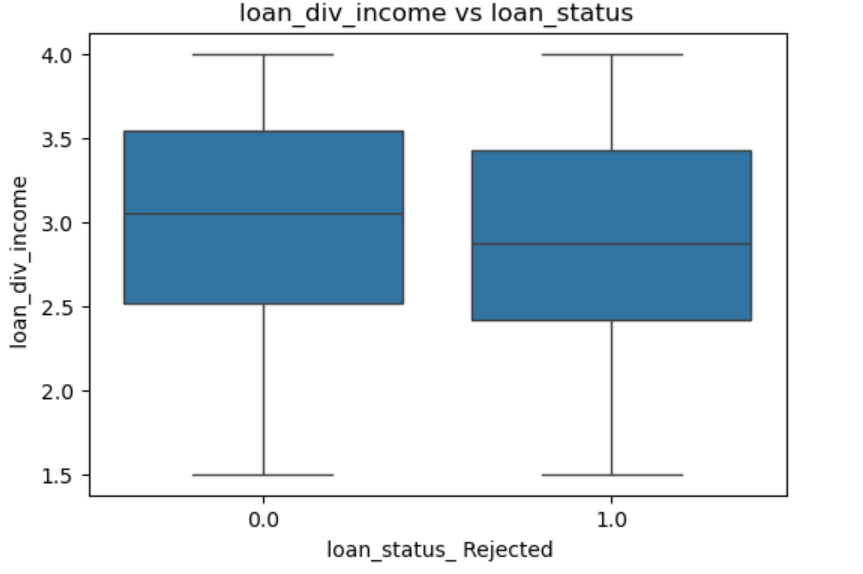

我们可以发现两边的数据分布差不多，所以两者并没有很强的相关性。我们当然还是可以放在后续步骤继续操作。

我们可以把现在数据包含的特征都打印出来，方便我们回顾一下。

print(df_processed.columns.tolist())

目前还是有11个特征，但我们数据预处理并没有完全结束。

5.3 数据标准化

数据预处理还需要对数据进行标准化，这样可以排除一些数据过大而主导整个模型。这么做也可以让模型收敛更快。一般来说这步操作都是必不可少的。

任务3.3让我们进行数据标准化。

我将其放在了特征工程之后也是为了方便我们在添加完特征后不需要进行重复的数据标准化操作。这么做更符合正常的流程。

相关的代码如下。

# Normalization is needed by our models
from sklearn.preprocessing import StandardScaler
# Select the numerical features that need to be normalized
numerical_features = [
    ' no_of_dependents',
    ' income_annum',
    ' loan_amount',
    ' loan_term',
    ' cibil_score',
    ' total_assets',
    ' loan_div_income'
]
# Create a copy to avoid modifying the original DataFrame
df_before_scaling = df_processed[numerical_features].copy()
# Create StandardScaler
scaler = StandardScaler()
df_processed[numerical_features] = scaler.fit_transform(df_processed[numerical_features])
print("Normalization done")

这里最后打印Normalization done可以让我们清楚知道这一步操作成功结束了。

5.4 训练集和测试集的划分

任务3.4要求我们进行数据划分。

这一步操作相对来说也很简单，我们将数据集分成1：4，百分之20用于测试，另外百分之80用于训练。

代码如下。

X = df_processed.drop(' loan_status_ Rejected', axis=1) # Replace 'Loan_Status' with the actual encoded target column name
y = df_processed[' loan_status_ Rejected'] # Replace 'Loan_Status' with the actual encoded target column name

X_train, X_test, y_train, y_test = train_test_split(X, y, test_size=0.2, random_state=42)

print("Shape of X_train:", X_train.shape)
print("Shape of X_test:", X_test.shape)
print("Shape of y_train:", y_train.shape)
print("Shape of y_test:", y_test.shape)

# Verify if there is a correspondence
if len(X_train) == len(y_train) and len(X_test) == len(y_test):
    print("Data Splitting Correct")
else:
    print("Data Splitting Incorrect")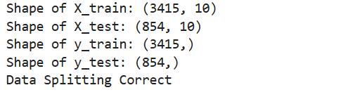

这里输出项括号里的第二个是特征数。y没有值是因为y是一维数据，因此这里的输出是正常的。

7. 模型选择和训练

我们需要选择一定数量的分类模型从而在训练集上训练数据以获得一个可以进行贷款批准预测的模型。

7.1 初始化以及训练模型

任务5.1要求我们需要训练三个模型出来。我选择了3个模型：逻辑回归（Logistic Regression）、决策树（Decision Tree Classifier）、随机森林（Random Forest Classifier）。

这里第一个模型是因为其简单，适合用于二元分类。而这里正是二元分类问题（Approved、Rejected），因此我们这里使用它来尝试。

之前的逻辑回归是一个线性模型，可能无法解决非线性类问题。我们这里前面发现过我们可以根据信用分来快速区分，这也是我们使用决策树的理由。

第三个模型我选择了一个集成分类器，它跟前面两个单一分类器相比通常具有更高的性能与泛化能力。因此我们现在确定了三个模型，下面就是分别训练它们，这里每个都有大量的超参数可以选择，我们这里没必要每个参数都进行大量的调试和选择，我们可以选择一些关键的进行网格搜索，下面的代码给出了参考。

逻辑回归：

from sklearn.linear_model import LogisticRegression
from sklearn.model_selection import GridSearchCV
model_lr = LogisticRegression(
    random_state=42, 
    solver='liblinear',
    max_iter=1000
)
model_lr.fit(X_train, y_train)

# Hyperparameter Tuning
# Define the parameter grid to be tuned
param_grid = {
    'C': [0.001, 0.01, 0.1, 1, 10, 100],  # Regularization Strength
    'penalty': ['l1', 'l2'],  # Regularization Type
    'solver': ['liblinear', 'saga'],  # Optimization Algorithm
    'max_iter': [500, 1000, 1500] # Iterator
}

# Create GridSearchCV object
grid_search = GridSearchCV(
    estimator=LogisticRegression(random_state=42),
    param_grid=param_grid,
    cv=5,
    scoring='accuracy',
    n_jobs=-1,
    verbose=1
)
grid_search.fit(X_train, y_train)
print("Best params (LR):", grid_search.best_params_)
print("Best CV score (LR):", grid_search.best_score_)
best_lr_model = grid_search.best_estimator_

决策树：

from sklearn.tree import DecisionTreeClassifier
model_dt = DecisionTreeClassifier(
    random_state=42,
    max_depth=5,
    min_samples_split=10
)
model_dt.fit(X_train, y_train)

# Hyperparameter Tuning
# Define the parameter grid to be tuned
dt_param_grid = {
    'max_depth': [3, 5, 7, 10, 15, 20, None], # Tree depth
    'min_samples_split': [2, 5, 10, 15, 20], # Minimum samples to split node
    'min_samples_leaf': [1, 2, 4, 6, 8, 10], # Minimum samples at leaf node
    'criterion': ['gini', 'entropy'], # Split criterion
    'max_features': ['sqrt', 'log2', None], # Number of features to consider
    'splitter': ['best', 'random'] # Split strategy
}

# Create GridSearchCV object
dt_grid_search = GridSearchCV(
    estimator=DecisionTreeClassifier(random_state=42),
    param_grid=dt_param_grid,
    cv=5,
    scoring='accuracy',
    n_jobs=-1,
    verbose=1,
)
dt_grid_search.fit(X_train, y_train)
print("Best params (DT):", dt_grid_search.best_params_)
print("Best CV score (DT):", dt_grid_search.best_score_)
best_dt_model = dt_grid_search.best_estimator_

随机森林：

from sklearn.ensemble import RandomForestClassifier
from sklearn.model_selection import RandomizedSearchCV
model_rf = RandomForestClassifier(
    random_state=42,
    n_estimators=100,  # Number of trees
    max_depth=10, # Maximum depth of each tree
    min_samples_split=10, # Minimum samples to split node
    min_samples_leaf=5, # Minimum samples at leaf node
    max_features='sqrt', # Number of features for best split
    bootstrap=True, # Use bootstrap sampling
    n_jobs=-1 # Use all available cores
)

model_rf.fit(X_train, y_train)

# Hyperparameter Tuning
# Define the parameter grid to be tuned
rf_param_dist = {
    'n_estimators': [50, 100, 200, 300, 400], # Number of trees
    'max_depth': [5, 10, 15, 20, 25, 30, None], # Maximum depth
    'min_samples_split': [2, 5, 10, 15, 20],  # Minimum samples to split
    'min_samples_leaf': [1, 2, 4, 6, 8], # Minimum samples at leaf
    'max_features': ['sqrt', 'log2', None, 0.5, 0.7], # Features to consider
    'bootstrap': [True, False], # Bootstrap sampling
    'criterion': ['gini', 'entropy'], # Split criterion
}

# Use RandomizedSearchCV for Random Forest (more efficient)
rf_random_search = RandomizedSearchCV(
    estimator=RandomForestClassifier(random_state=42),
    param_distributions=rf_param_dist,
    n_iter=50,
    cv=5,
    scoring='accuracy',
    random_state=42,
    n_jobs=-1,
    verbose=1,
    refit=True
)
rf_random_search.fit(X_train, y_train)
print("Best params (DT):", rf_random_search.best_params_)
print("Best CV score (DT):", rf_random_search.best_score_)
best_rf_model = rf_random_search.best_estimator_

8. 模型评估

训练完模型就要对这些训练好的模型进行评估。

8.1评估过程

任务6.1要求我们用测试集对这些模型进行测试。

from sklearn.metrics import accuracy_score, precision_score, recall_score, f1_score, roc_auc_score, confusion_matrix

y_pred_lr = best_lr_model.predict(X_test)
y_prob_lr = best_lr_model.predict_proba(X_test)[:, 1]
y_pred_dt = best_dt_model.predict(X_test)
y_prob_dt = best_dt_model.predict_proba(X_test)[:, 1]
y_pred_rf = best_rf_model.predict(X_test)
y_prob_rf = best_rf_model.predict_proba(X_test)[:, 1]

然后后续的三个任务让我们将这些结果分别清晰地展示出来。

任务6.2展示模型1结果。

这里将正确率，两个类别的精确率、召回率、F1分数，ROC AUC以及混淆矩阵全部都计算并打印了出来。

对于混淆矩阵还专门做了一个可视化从而更清晰展现数据。后续的任务6.3和6.4也是类似。

# Print Accuracy
print("Tuned LR - Accuracy:", accuracy_score(y_test, y_pred_lr))

# Print results of Approved
print("\nTuned LR - Approved  (0):")
print("Precision:", precision_score(y_test, y_pred_lr, pos_label=0))
print("Recall:", recall_score(y_test, y_pred_lr, pos_label=0))
print("F1:", f1_score(y_test, y_pred_lr, pos_label=0))

# Print results of Rejected
print("\nTuned LR - Rejected  (1):")
print("Precision:", precision_score(y_test, y_pred_lr, pos_label=1))
print("Recall:", recall_score(y_test, y_pred_lr, pos_label=1))
print("F1:", f1_score(y_test, y_pred_lr, pos_label=1))

# Print ROC AUC
print("\nTuned LR - ROC AUC:", roc_auc_score(y_test, y_prob_lr))

# Print the confusion matrix
print("\nTuned LR - Confusion Matrix [[Approved],[Rejected]]:")
print(confusion_matrix(y_test, y_pred_lr))

# Show the confusion matrix
cm = confusion_matrix(y_test, y_pred_lr)
labels = ['Approved (0)', 'Rejected (1)']
plt.figure(figsize=(10, 8))
sns.heatmap(cm, 
            annot=True, 
            fmt='d',
            cmap='Blues', 
            xticklabels=labels, 
            yticklabels=labels)

plt.title('Tuned Logistic Regression - Confusion Matrix', fontsize=16, pad=20)
plt.xlabel('Predicted Label', fontsize=14)
plt.ylabel('True Label', fontsize=14)
plt.tight_layout()
plt.show()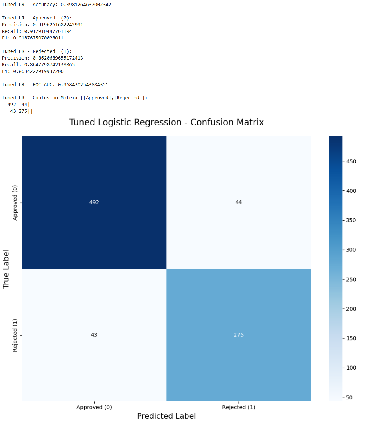

任务6.3是模型2的结果。

# Print Accuracy
print("Tuned DT - Accuracy:", accuracy_score(y_test, y_pred_dt))

# Print results of Approved
print("\nTuned DT - Approved  (0):")
print("Precision:", precision_score(y_test, y_pred_dt, pos_label=0))
print("Recall:", recall_score(y_test, y_pred_dt, pos_label=0))
print("F1:", f1_score(y_test, y_pred_dt, pos_label=0))

# Print results of Rejected
print("\nTuned DT - Rejected  (1):")
print("Precision:", precision_score(y_test, y_pred_dt, pos_label=1))
print("Recall:", recall_score(y_test, y_pred_dt, pos_label=1))
print("F1:", f1_score(y_test, y_pred_dt, pos_label=1))

# Print ROC AUC
print("\nTuned DT - ROC AUC:", roc_auc_score(y_test, y_prob_dt))

# Print the confusion matrix
print("\nTuned DT - Confusion Matrix [[Approved],[Rejected]]:")
print(confusion_matrix(y_test, y_pred_dt))

# Show the confusion matrix
cm = confusion_matrix(y_test, y_pred_dt)
labels = ['Approved (0)', 'Rejected (1)']
plt.figure(figsize=(10, 8))
sns.heatmap(cm, 
            annot=True, 
            fmt='d',
            cmap='Blues', 
            xticklabels=labels, 
            yticklabels=labels)

plt.title('Tuned Decision Tree - Confusion Matrix', fontsize=16, pad=20)
plt.xlabel('Predicted Label', fontsize=14)
plt.ylabel('True Label', fontsize=14)
plt.tight_layout()
plt.show()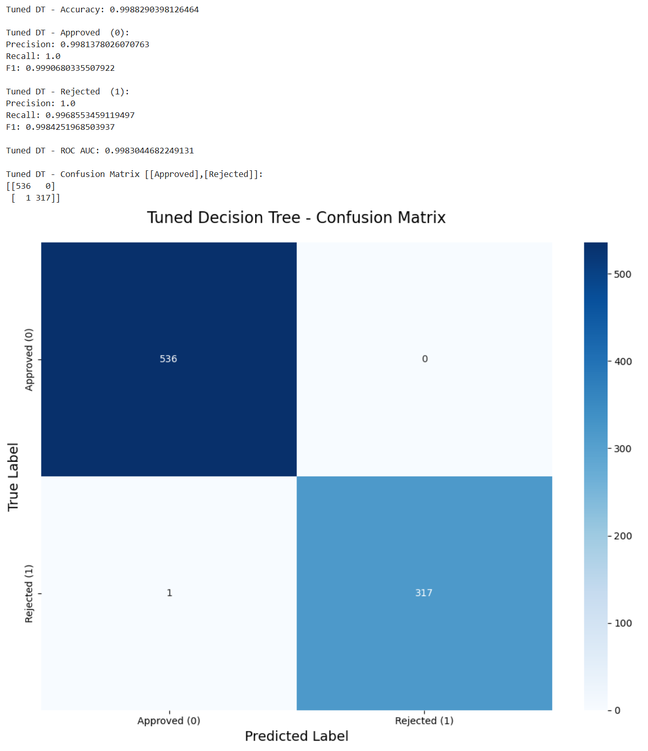

第三个模型如下。

# Print Accuracy
print("Tuned RF - Accuracy:", accuracy_score(y_test, y_pred_rf))

# Print results of Approved
print("\nTuned RF - Approved  (0):")
print("Precision:", precision_score(y_test, y_pred_rf, pos_label=0))
print("Recall:", recall_score(y_test, y_pred_rf, pos_label=0))
print("F1:", f1_score(y_test, y_pred_rf, pos_label=0))

# Print results of Rejected
print("\nTuned RF - Rejected  (1):")
print("Precision:", precision_score(y_test, y_pred_rf, pos_label=1))
print("Recall:", recall_score(y_test, y_pred_rf, pos_label=1))
print("F1:", f1_score(y_test, y_pred_rf, pos_label=1))

# Print ROC AUC
print("\nTuned RF - ROC AUC:", roc_auc_score(y_test, y_prob_rf))

# Print the confusion matrix
print("\nTuned RF - Confusion Matrix [[Approved],[Rejected]]:")
print(confusion_matrix(y_test, y_pred_rf))

# Show the confusion matrix
cm = confusion_matrix(y_test, y_pred_rf)
labels = ['Approved (0)', 'Rejected (1)']
plt.figure(figsize=(10, 8))
sns.heatmap(cm, 
            annot=True, 
            fmt='d',
            cmap='Blues', 
            xticklabels=labels, 
            yticklabels=labels)

plt.title('Tuned Random Forest - Confusion Matrix', fontsize=16, pad=20)
plt.xlabel('Predicted Label', fontsize=14)
plt.ylabel('True Label', fontsize=14)
plt.tight_layout()
plt.show()

8.2 评估比较

我们现在对这些评估的结果进行比较从而得出更深一步的结论。

任务6.4正是让我们进行比较和讨论。

我们首先可以发现的是决策树和随机森林模型都可以很好地预测贷款状态。两者都有99%的准确率。然而，逻辑回归的准确率为89%。这表明该问题仍然可以通过线性模型来解决，但由于线性模型的局限性，它不能完全拟合。

我们回到这个任务的更深层次的目的上，我们的任务是帮助开发一个贷款批准的预测模型，这么做是希望避免银行的经济损失。因此假阳性是模型错误预测为阳性的样本数量，这里意味着批准了不正确的人，这将导致直接的经济损失。在这种情况下，虚假否定是拒绝应该获得贷款的人，这减少了银行的一些利润，这是一种间接的经济损失。因此，在这种情况下，银行应该更加重视拒收的准确性。

而我们现在决策树和随机森林有相同的性能，我们可以根据特征重要性来确定这两个模型是否是同一个模型。以下代码实现了此功能。

dt_importance = best_dt_model.feature_importances_
rf_importance = best_rf_model.feature_importances_

dt_top_idx = np.argsort(dt_importance)[-5:][::-1]
rf_top_idx = np.argsort(rf_importance)[-5:][::-1]

print("The 5 most important features of Decision Trees：")
for idx in dt_top_idx:
    print(f"  {X.columns[idx]}: {dt_importance[idx]:.4f}")

print("\nThe 5 most important features of Random Forest：")
for idx in rf_top_idx:
    print(f"  {X.columns[idx]}: {rf_importance[idx]:.4f}")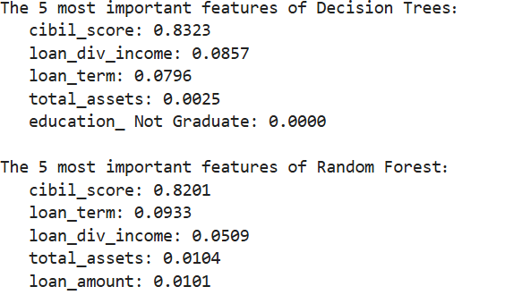

我们可以清晰地发现两者的组成并不相同，因此它们并不是完全相同的模型。

我们还可以发现这两个模型对CIBIL评分的特征重要性最高。这与我们之前的预测一致，即CIBIL评分和贷款状态之间存在很强的相关性。我们还可以考虑到实际情况，CIBIL评分直接反映了客户的信用历史和还款能力，这确实可以成为预测贷款批准的决定性特征。

而我们现在这两个模型不同但又评估结果相同，因此为了选择出最佳的模型我们恐怕需要更多的数据进行评估。

这里能给到银行的建议如下：

1. 如果优先考虑可解释性和合规性：决策树。
2. 如果优先考虑稳定性和准确性：随机森林。

9. 总结

我们现在总结一下我们的整个项目，这里老师同样给出了思路。

任务7.1让我们再总结一下我们的发现。

我们可以发现CIBIL评分在贷款审批中起着至关重要的作用。由于其关键作用，即使是像逻辑回归这样的线性模型也能以89%的准确率预测结果。决策树和随机森林的准确率达到99%。这三个模型都能很好地预测贷款状况。

任务7.2让我们说一下最优模型和见解。

在我们的项目中，决策树和随机森林模型在多种标准下都取得了同样出色的性能。如果我们考虑实际情况，以项目的精度为标准，这两个模型都符合核心业务要求。通过分析它们的特征重要性，我们确定这两个模型并不完全一致。

因此，我们今后只能根据实际情况选择这两种模式。如果我们希望模型具有更高的准确性，我们可以选择随机森林。如果我们想要更低的运营成本和更好的可解释性，我们可以选择决策树。

任务7.3需要我们给出建议以及未来工作的方向。

这一点我们刚刚也提到了。

由于我们最后两个模型的性能一致，我们未来的工作是收集更多数据进行更多测试或进行更多交叉验证该模型可以在不同的列车测试分段下进行测试，也可以通过重复的交叉验证来确认稳定性。此外，我们可以从不同时期收集相关数据，以提高我们模型的适应性。

当然我只是提到了整体上的思路，具体的细节都可以查看我的最后的结果 作业示例。这里面还解释了每个方法的优点和缺点，以及这么做是为什么，这样更能提现对这些知识的理解。