【3D-AICG 系列-13】Trellis 2 的 SC-VAE 的 Training Loss 细节

系列文章目录

• 【3D AICG 系列-1】Trellis v1 和 Trellis v2 的区别和改进
• 【3D AICG 系列-2】Trellis 2 的O-voxel (上) Shape: Flexible Dual Grid
• 【3D AICG 系列-3】Trellis 2 的O-voxel (下) Material: Volumetric Surface Attributes
• 【3D AICG 系列-4】Trellis 2 的Shape SLAT Flow Matching DiT 训练流程
• 【3D AICG 系列-5】Trellis 2 的 Pipeline 推理流程的各个中间结果和形状
• 【3D AICG 系列-6】OmniPart 训练流程梳理
• 【3D AICG 系列-7】PartUV 代码流程深度解析
• 【3D AICG 系列-8】PartUV 流程图详解
• 【3D AICG 系列-9】Trellis2 推理流程图超详细介绍
• 【3D-AICG 系列-10】Trellis v2 只在 512/1024上训却能生成 1536
• 【3D-AICG 系列-11】Trellis 2 的 Shape VAE 训练流程梳理
• 【3D-AICG 系列-12】Trellis 2 的 Shape VAE 的设计细节 Sparse Residual Autoencoding Layer

文章目录

• 系列文章目录
• • • 一、符号与变量对应
    • [二、第一阶段损失 L s 1 \mathcal{L}{s1} Ls1（公式 6）](#二、第一阶段损失 L s 1 \mathcal{L}{s1} Ls1（公式 6）)
    • • [1. λ v ∥ v ^ − v ∥ 2 2 \lambda_v \|\hat{v}-v\|_2^2 λv∥v^−v∥22（对偶顶点 MSE）](#1. λ v ∥ v ^ − v ∥ 2 2 \lambda_v |\hat{v}-v|_2^2 λv∥v^−v∥22（对偶顶点 MSE）)
      • [2. λ δ BCE ( δ ^ , δ ) \lambda_\delta \text{BCE}(\hat{\delta},\delta) λδBCE(δ^,δ)（对偶面标志 BCE）](#2. λ δ BCE ( δ ^ , δ ) \lambda_\delta \text{BCE}(\hat{\delta},\delta) λδBCE(δ^,δ)（对偶面标志 BCE）)
      • [3. λ ρ BCE ( ρ ^ , ρ ) \lambda_\rho \text{BCE}(\hat{\rho},\rho) λρBCE(ρ^,ρ)（剪枝/细分掩码 BCE）](#3. λ ρ BCE ( ρ ^ , ρ ) \lambda_\rho \text{BCE}(\hat{\rho},\rho) λρBCE(ρ^,ρ)（剪枝/细分掩码 BCE）)
      • [4. λ mat ∥ f ^ mat − f mat ∥ 1 \lambda_{\text{mat}}\|\hat{f}^{\text{mat}}-f^{\text{mat}}\|1 λmat∥f^mat−fmat∥1（材质 L1）](#4. λ mat ∥ f ^ mat − f mat ∥ 1 \lambda{\text{mat}}|\hat{f}^{{\text{mat}}-f}{\text{mat}}|_1 λmat∥f^mat−fmat∥1（材质 L1）)
      • [5. λ K L L K L \lambda_{KL}\mathcal{L}{KL} λKLLKL](#5. λ K L L K L \lambda{KL}\mathcal{L}_{KL} λKLLKL)
    • [三、第二阶段损失 L s 2 = L s 1 + L render \mathcal{L}{s2} = \mathcal{L}{s1} + \mathcal{L}{\text{render}} Ls2=Ls1+Lrender（公式 7）](#三、第二阶段损失 L s 2 = L s 1 + L render \mathcal{L}{s2} = \mathcal{L}{s1} + \mathcal{L}{\text{render}} Ls2=Ls1+Lrender（公式 7）)
    • 四、相机策略（浅近裁剪平面）
    • [五、解耦潜在空间：材质以 shape 的细分结构为条件](#五、解耦潜在空间：材质以 shape 的细分结构为条件)
    • 六、汇总表

本文是论文 3.2.2 VAE Training 与代码的逐项对应说明。

---

一、符号与变量对应

论文符号	含义	代码变量 / 说明
v v v	对偶顶点位置	vertices（dual grid 顶点偏移，3 维）
δ \delta δ	对偶面/边标志	intersected（体素 3 条边是否被面穿过，3 维 bool）
ρ \rho ρ	剪枝/细分掩码	subdivision ：上采样时"是否在该 coarse 下生成 8 个子体素"的 mask，即 subs_gt / subs
f mat f^{\text{mat}} fmat	材质属性	PBR VAE 的 x.feats（base_color, metallic, roughness, alpha 等）
v ^ \hat{v} v^	预测值	decoder 输出：pred_vertice, pred_intersected, subs, 以及 PBR 的 y.feats

---

二、第一阶段损失 L s 1 \mathcal{L}_{s1} Ls1（公式 6）

论文：

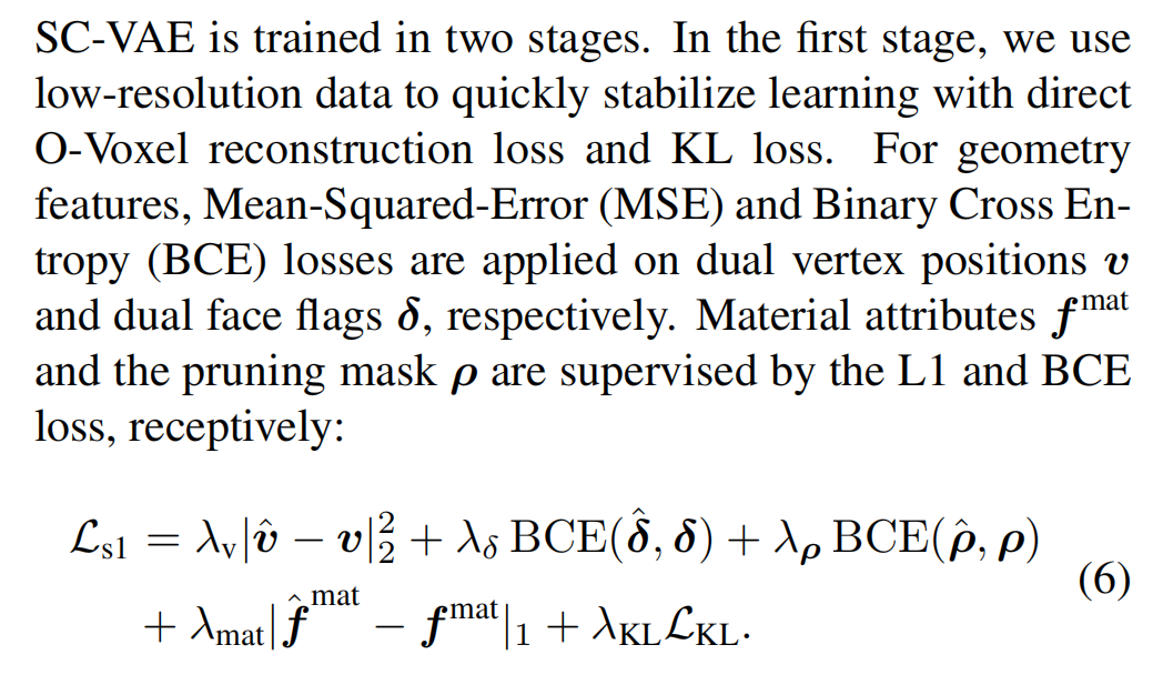
1. λ v ∥ v ^ − v ∥ 2 2 \lambda_v \|\hat{v}-v\|_2^2 λv∥v^−v∥22（对偶顶点 MSE）

代码： ShapeVaeTrainer，lambda_vertice（默认 0.01）

        if self.lambda_vertice > 0:
            terms["direct/vertice"] = F.mse_loss(pred_vertice.feats, vertices.feats)
            terms["loss"] = terms["loss"] + self.lambda_vertice * terms["direct/vertice"]

• 论文 v v v ↔ vertices.feats， v ^ \hat{v} v^ ↔ pred_vertice.feats
• 实现就是 MSE，等价于 ∥ v ^ − v ∥ 2 2 \|\hat{v}-v\|_2^2 ∥v^−v∥22 的 mean

2. λ δ BCE ( δ ^ , δ ) \lambda_\delta \text{BCE}(\hat{\delta},\delta) λδBCE(δ^,δ)（对偶面标志 BCE）

代码： lambda_intersected（默认 0.1）

        if self.lambda_intersected > 0:
            terms["direct/intersected"] = F.binary_cross_entropy_with_logits(pred_intersected.feats.flatten(), intersected.feats.flatten().float())
            terms["loss"] = terms["loss"] + self.lambda_intersected * terms["direct/intersected"]

• 论文 δ \delta δ ↔ intersected， δ ^ \hat{\delta} δ^ ↔ pred_intersected（logits）
• 用 binary_cross_entropy_with_logits 即 BCE

3. λ ρ BCE ( ρ ^ , ρ ) \lambda_\rho \text{BCE}(\hat{\rho},\rho) λρBCE(ρ^,ρ)（剪枝/细分掩码 BCE）

代码： subdivision 预测的 BCE，lambda_subdiv（默认 0.1）

        for i, (sub_gt, sub) in enumerate(zip(subs_gt, subs)):
            terms[f"bce_sub{i}"] = F.binary_cross_entropy_with_logits(sub.feats, sub_gt.float())
            terms["loss"] = terms["loss"] + self.lambda_subdiv * terms[f"bce_sub{i}"]

• 论文 ρ \rho ρ ↔ 每层上采样的 GT subdivision subs_gt（来自 encoder 下采样时的 spatial cache）
• ρ ^ \hat{\rho} ρ^ ↔ decoder 每层预测的 subs
• 多层累加，每层权重都是 lambda_subdiv

4. λ mat ∥ f ^ mat − f mat ∥ 1 \lambda_{\text{mat}}\|\hat{f}^{\text{mat}}-f^{\text{mat}}\|_1 λmat∥f^mat−fmat∥1（材质 L1）

代码： 在 PBR VAE 里，对应 direct regression 的 L1

        if self.loss_type == 'l1':
            terms["l1"] = l1_loss(x.feats, y.feats)
            terms["loss"] = terms["loss"] + terms["l1"]
        elif self.loss_type == 'l2':
            terms["l2"] = l2_loss(x.feats, y.feats)
            terms["loss"] = terms["loss"] + terms["l2"]

• f mat f^{\text{mat}} fmat ↔ x.feats， f ^ mat \hat{f}^{\text{mat}} f^mat ↔ y.feats
• 论文写的是 L1，配置里用 loss_type='l1' 时就是 ∥ f ^ mat − f mat ∥ 1 \|\hat{f}^{\text{mat}}-f^{\text{mat}}\|_1 ∥f^mat−fmat∥1

5. λ K L L K L \lambda_{KL}\mathcal{L}_{KL} λKLLKL

代码： 两个 VAE 都用同一形式的 KL

Shape VAE：

        terms["kl"] = 0.5 * torch.mean(mean.pow(2) + logvar.exp() - logvar - 1)
        terms["loss"] = terms["loss"] + self.lambda_kl * terms["kl"]

PBR VAE：

        terms["kl"] = 0.5 * torch.mean(mean.pow(2) + logvar.exp() - logvar - 1)
        terms["loss"] = terms["loss"] + self.lambda_kl * terms["kl"]

• 即标准高斯先验的 KL： 1 2 ( μ 2 + e log ⁡ σ 2 − log ⁡ σ 2 − 1 ) \frac{1}{2}(\mu^2 + e^{\log\sigma^2} - \log\sigma^2 - 1) 21(μ2+elogσ2−logσ2−1)
• Shape 配置里 lambda_kl=1e-6，很小，符合"第一阶段以重建为主"的写法

---

三、第二阶段损失 L s 2 = L s 1 + L render \mathcal{L}{s2} = \mathcal{L}{s1} + \mathcal{L}_{\text{render}} Ls2=Ls1+Lrender（公式 7）

论文：第二阶段在 L s 1 \mathcal{L}_{s1} Ls1 上再加基于渲染的感知损失。

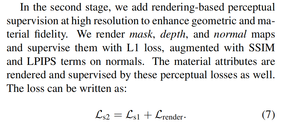
代码： 没有拆成两个训练阶段，而是在同一个 training_losses() 里同时算 direct + 渲染，对应"始终在用 L s 2 \mathcal{L}_{s2} Ls2"：

        # rendering loss
        cameras = self._randomize_camera(len(mesh))
        gt_renders = self._render_batch(mesh, **cameras, return_types=['mask', 'normal', 'depth'])
        pred_renders = self._render_batch(recon, **cameras, return_types=['mask', 'normal', 'depth'])
        terms['render/mask'] = l1_loss(pred_renders['mask'], gt_renders['mask'])
        terms['render/depth'] = l1_loss(pred_renders['depth'], gt_renders['depth'])
        terms['render/normal/l1'] = l1_loss(pred_renders['normal'], gt_renders['normal'])
        terms['render/normal/ssim'] = 1 - ssim(pred_renders['normal'], gt_renders['normal'])
        terms['render/normal/lpips'] = lpips(pred_renders['normal'], gt_renders['normal'])
        terms['loss'] = terms["loss"] + \
                        self.lambda_mask * terms['render/mask'] + \
                        self.lambda_depth * terms['render/depth'] + \
                        self.lambda_normal * (terms['render/normal/l1'] + self.lambda_ssim * terms['render/normal/ssim'] + self.lambda_lpips * terms['render/normal/lpips'])

对应关系：

论文描述	代码
渲染 mask	return_types=['mask', ...]，L1，权重 lambda_mask=1
渲染 depth	return_types=['depth', ...]，L1，权重 lambda_depth=10
法线 L1	terms['render/normal/l1']，权重 lambda_normal=1
法线 SSIM	terms['render/normal/ssim']，权重 lambda_normal * lambda_ssim（0.2）
法线 LPIPS	terms['render/normal/lpips']，权重 lambda_normal * lambda_lpips（0.2）

若要"只做第一阶段"，可在配置里把 lambda_mask、lambda_depth、lambda_normal 设为 0，即退化为 L s 1 \mathcal{L}_{s1} Ls1。

材质 VAE 的"第二阶段"是渲染感知损失（base_color / MRA 的 SSIM+LPIPS）：

            terms['render/base_color/ssim'] = 1 - ssim(pred_base_color, gt_base_color)
            terms['render/base_color/lpips'] = lpips(pred_base_color, gt_base_color)
            terms['render/mra/ssim'] = 1 - ssim(pred_mra, gt_mra)
            terms['render/mra/lpips'] = lpips(pred_mra, gt_mra)
            terms['loss'] = terms["loss"] + \
                            self.lambda_render * (self.lambda_ssim * ... + self.lambda_lpips * ...)

对应论文里"材质也通过感知损失监督"。

---

四、相机策略（浅近裁剪平面）

论文：随机放置相机，并用浅的近裁剪平面"切开"物体表面，以建模内外结构。

代码： ShapeVaeTrainer._randomize_camera：

        r_min, r_max = self.camera_randomization_config['radius_range']
        k_min = 1 / r_max**2
        k_max = 1 / r_min**2
        ks = torch.rand(num_samples, device=self.device) * (k_max - k_min) + k_min
        radius = 1 / torch.sqrt(ks)
        fov = 2 * torch.arcsin(0.5 / radius)
        origin = radius.unsqueeze(-1) * F.normalize(torch.randn(num_samples, 3, device=self.device), dim=-1)
        extrinsics = utils3d.torch.extrinsics_look_at(origin, torch.zeros_like(origin), ...)
        intrinsics = utils3d.torch.intrinsics_from_fov_xy(fov, fov)
        near = [np.random.uniform(r - 1, r) for r in radius.tolist()]
        return { 'extrinsics': ..., 'intrinsics': ..., 'near': near }

• radius_range: [2, 100]：相机到原点的距离在 [2, 100] 内随机（在 1/k 空间均匀）。
• near 取在 [radius - 1, radius]，即近平面紧贴相机、远平面 far = near + 2，形成很薄的视锥，相当于用近平面"切"过物体，对应论文的 shallow near plane 和"切开表面、看到内外结构"。

---

五、解耦潜在空间：材质以 shape 的细分结构为条件

论文：两个解耦的 SC-VAE（shape + material），材质 VAE 上采样时以 shape VAE 的 subdivision structures 为条件。

代码： 推理时，纹理 decoder 显式接收 shape 的 subdivision 作为 guide_subs：

        ret = self.models['tex_slat_decoder'](slat, guide_subs=subs) * 0.5 + 0.5

• subs 来自 shape 的 decoder 在上采样时返回的 subdivision 列表（每层"哪些 coarse 体素被细分为 8 个子体素"）。
• 纹理 decoder 若 pred_subdiv=False，则使用 guide_subs 决定在哪些位置做 channel→spatial 上采样，从而与 shape 的几何结构对齐。

Decoder 接口（支持 guide_subs）：

    def forward(self, x: sp.SparseTensor, guide_subs: Optional[List[sp.SparseTensor]] = None, return_subs: bool = False) -> sp.SparseTensor:
        assert guide_subs is None or self.pred_subdiv == False, "Only decoders with pred_subdiv=False can be used with guide_subs"

因此：论文里的 "subdivision structures" = 代码里的 subs / `guide_subs；材质/纹理 decoder 在推理（和可选的训练）时按 shape 的细分结构做条件上采样。

---

六、汇总表

论文公式/概念	代码位置	配置/权重
λ v ∣ v ^ − v ∣ 2 2 \lambda_v |\hat{v}-v|_2^2 λv∣v^−v∣22	shape_vae.py L189-190	lambda_vertice=0.01
λ δ BCE ( δ ^ , δ ) \lambda_\delta \text{BCE}(\hat{\delta},\delta) λδBCE(δ^,δ)	shape_vae.py 第186-188行	lambda_intersected=0.1
λ ρ BCE ( ρ ^ , ρ ) \lambda_\rho \text{BCE}(\hat{\rho},\rho) λρBCE(ρ^,ρ)	shape_vae.py 第193-195行	lambda_subdiv=0.1
λ mat ∣ f ^ mat − f mat ∣ 1 \lambda_{\text{mat}}|\hat{f}^{\text{mat}}-f^{\text{mat}}|_1 λmat∣f^mat−fmat∣1	pbr_vae.py 第175-177行	loss_type='l1'
λ K L L K L \lambda_{KL}\mathcal{L}_{KL} λKLLKL	shape_vae.py 第211-213行；pbr_vae.py 第217-219行	lambda_kl=1e-6
L render \mathcal{L}_{\text{render}} Lrender（mask/depth 损失）	shape_vae.py 第200-206行	lambda_mask=1、lambda_depth=10
法线 L1 + SSIM + LPIPS	shape_vae.py L202-208	lambda_normal=1, lambda_ssim/lpips=0.2
材质渲染感知损失	pbr_vae.py L208-214	lambda_render, lambda_ssim, lambda_lpips
随机相机 + 浅 near	shape_vae.py L113-126，camera_randomization_config	radius_range=[2,100], near ∈ [r-1,r]
材质以 subdivision 为条件	tex_slat_decoder(..., guide_subs=subs)，decoder forward(..., guide_subs=...)	pipeline / sparse_unet_vae

这样就把论文 3.2.2 的公式、两阶段、相机和"材质条件于 shape 细分结构"都和代码对上去了。