异或问题（XOR Question）：从单层感知机到多层感知机

XOR问题是计算机科学和人工智能领域的经典问题，主要用于研究逻辑运算和神经网络的能力，其目标是让神经网络学会异或运算：

真值表

输入1	输入2	输出
0	0	0
1	0	1
0	1	1
1	1	0

认识XOR问题

XOR问题是线性不可分的，单层感知机学不会，必须有多层、非线性激活。下面我们来逐一学习其中的基本概念。

线性可分性

一、基础概念：线性决策边界

在深度学习中，分类问题的核心是找到一个决策边界（Decision Boundary），将不同类别的样本分开。

线性决策边界：指可以用一条直线（二维平面）或一个平面（三维空间）来完美分隔不同类别的样本。

非线性决策边界：需要更复杂的曲线或曲面才能分隔样本。

二、线性可分问题（`Linearly Separable`）

1. 定义

如果存在一条直线（或超平面），使得所有正类样本 和负类样本 分别位于该直线的两侧，则称该问题是线性可分的。

2. 数学表示

假设样本特征为 <math xmlns="http://www.w3.org/1998/Math/MathML"> x = [ x 1 , x 2 ] T \boldsymbol{x} = [x_1, x_2]^T </math>x=[x1,x2]T，标签 <math xmlns="http://www.w3.org/1998/Math/MathML"> y ∈ { + 1 , − 1 } y \in \{+1, -1\} </math>y∈{+1,−1}。线性决策边界可表示为： <math xmlns="http://www.w3.org/1998/Math/MathML"> w T x + b = 0 \boldsymbol{w}^T \boldsymbol{x} + b = 0 </math>wTx+b=0

其中 <math xmlns="http://www.w3.org/1998/Math/MathML"> w \boldsymbol{w} </math>w是权重向量， <math xmlns="http://www.w3.org/1998/Math/MathML"> b b </math>b是偏置项。

分类规则为：

<math xmlns="http://www.w3.org/1998/Math/MathML"> y = { + 1 , w T x + b > 0 − 1 , w T x + b < 0 y=\left\{\begin{matrix} +1, \boldsymbol{w}^T\boldsymbol{x} + b > 0& \\ -1, \boldsymbol{w}^T\boldsymbol{x} + b < 0& \end{matrix}\right. </math>y={+1,wTx+b>0−1,wTx+b<0

即线性函数结果为正则为 <math xmlns="http://www.w3.org/1998/Math/MathML"> + 1 +1 </math>+1，否则为 <math xmlns="http://www.w3.org/1998/Math/MathML"> − 1 -1 </math>−1。

3. 示例

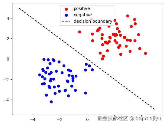
下图展示二维平面中的线性可分问题：

红色点（正类）和蓝色点（负类）可被一条直线完美分隔，是线性可分的。

python 复制代码

import matplotlib.pyplot as plt
import numpy as np

# 生成线性可分数据
np.random.seed(0)
X_pos = np.random.randn(50, 2) + [2, 2]    # 正类样本
X_neg = np.random.randn(50, 2) + [-2, -2]  # 负类样本

# 绘制决策边界 w=[1,1], b=0
x_bound = np.linspace(-5, 5, 100)
y_bound = -x_bound  # w1*x1 + w2*x2 =0 → x2 = -x1

plt.scatter(X_pos[:,0], X_pos[:,1], c='red', label='positive')
plt.scatter(X_neg[:,0], X_neg[:,1], c='blue', label='negative')
plt.plot(x_bound, y_bound, 'k--', label='decision boundary')
plt.legend()
plt.show()

运行结果：

三、线性不可分问题（`Linearly Inseparable`）

1. 定义

如果不存在任何直线（或超平面）能完美分隔所有样本，则称该问题是线性不可分的。

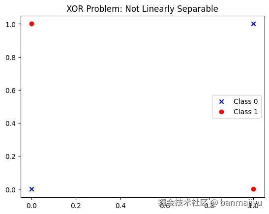
2. 典型例子：异或问题（XOR）

异或问题的样本分布如下：

输入1	输入2	输出
0	0	0
1	0	1
0	1	1
1	1	0

在二维平面上，样本点 <math xmlns="http://www.w3.org/1998/Math/MathML"> ( 0 , 0 ) (0,0) </math>(0,0)和 <math xmlns="http://www.w3.org/1998/Math/MathML"> ( 1 , 1 ) (1,1) </math>(1,1)属于一类， <math xmlns="http://www.w3.org/1998/Math/MathML"> ( 0 , 1 ) (0,1) </math>(0,1) 和 <math xmlns="http://www.w3.org/1998/Math/MathML"> ( 1 , 0 ) (1,0) </math>(1,0) 属于另一类。无法用一条直线分隔两类样本。

3. 可视化

python 复制代码

# 异或问题数据
X_xor = np.array([[0, 0], [0, 1], [1, 0], [1, 1]])
y_xor = np.array([0, 1, 1, 0])

plt.scatter(X_xor[y_xor==0, 0], X_xor[y_xor==0, 1], c='blue', marker='x', label='Class 0')
plt.scatter(X_xor[y_xor==1, 0], X_xor[y_xor==1, 1], c='red', marker='o', label='Class 1')
plt.title('XOR Problem: Not Linearly Separable')
plt.legend()
plt.show()

运行结果：

单层感知机

接下来我们将动手解决上述问题，我们先从最简单的线性可分问题 开始。解决线性可分问题需要用到单层感知机，这也是深度学习中最基础的模型之一。

一、什么是单层感知机？

单层感知机是一种二分类线性模型，它的核心思想是模拟生物神经元的工作方式：

输入：接收多个信号（特征）
处理：对输入加权求和，再通过激活函数
输出：生成一个二值结果（如 <math xmlns="http://www.w3.org/1998/Math/MathML"> 0 0 </math>0 / <math xmlns="http://www.w3.org/1998/Math/MathML"> 1 1 </math>1）

二、核心元件与数学原理

输入层（Input Layer）
- 作用：接收外部数据，例如 <math xmlns="http://www.w3.org/1998/Math/MathML"> n n </math>n个特征 <math xmlns="http://www.w3.org/1998/Math/MathML"> x 1 , x 2 , ... , x n x_1, x_2, \dots, x_n </math>x1,x2,...,xn
- 数学表示： <math xmlns="http://www.w3.org/1998/Math/MathML"> x = [ x 1 , x 2 , ... , x n ] \mathbf{x} = [x_1, x_2, \dots, x_n] </math>x=[x1,x2,...,xn]
权重（Weights）
- 作用：每个输入对应一个权重 <math xmlns="http://www.w3.org/1998/Math/MathML"> w i w_i </math>wi
- 数学表示： <math xmlns="http://www.w3.org/1998/Math/MathML"> w = [ w 1 , w 2 , ... , w n ] \mathbf{w} = [w_1, w_2, \dots, w_n] </math>w=[w1,w2,...,wn]
偏置（Bias）
- 作用：调整模型的灵活性，类似截距项。
- 符号： <math xmlns="http://www.w3.org/1998/Math/MathML"> b b </math>b（可视为 <math xmlns="http://www.w3.org/1998/Math/MathML"> w 0 w_0 </math>w0 对应固定输入 <math xmlns="http://www.w3.org/1998/Math/MathML"> x 0 = 1 x_0=1 </math>x0=1）
加权求和（Weighted Sum）
- 计算：输入与权重的线性组合： <math xmlns="http://www.w3.org/1998/Math/MathML"> z = ∑ i = 1 n w i x i + b z = \sum\limits_{i=1}^{n} w_i x_i + b </math>z=i=1∑nwixi+b
- 向量形式： <math xmlns="http://www.w3.org/1998/Math/MathML"> z = w T x + b z = \mathbf{w}^T \mathbf{x} + b </math>z=wTx+b （一个仿射变换）
激活函数（Activation Function）
- 作用：对信号作一次非线性变形。将连续值 <math xmlns="http://www.w3.org/1998/Math/MathML"> z z </math>z转换为二值输出（如 <math xmlns="http://www.w3.org/1998/Math/MathML"> 0 0 </math>0 或 <math xmlns="http://www.w3.org/1998/Math/MathML"> 1 1 </math>1 ）。
- 常用函数：
  - 阶跃函数（Step Function）： <math xmlns="http://www.w3.org/1998/Math/MathML"> y = { 1 , z > 0 0 , z ⩽ 0 y=\left\{\begin{matrix} 1,z> 0 & \\ 0,z \leqslant 0 & \end{matrix}\right. </math>y={1,z>00,z⩽0
  - Sigmoid： <math xmlns="http://www.w3.org/1998/Math/MathML"> f ( z ) = 1 1 + e − z f(z)=\dfrac{1}{1+e^{-z}} </math>f(z)=1+e−z1
  - ReLU： <math xmlns="http://www.w3.org/1998/Math/MathML"> f ( z ) = max ⁡ ( 0 , z ) f(z)=\max(0,z) </math>f(z)=max(0,z)

一个单层感知机就是一个神经元

三、决策边界

单层感知机的本质是找到一个线性决策边界：

功能：将输入空间划分为两个区域（如正类和负类）。
限制：只能解决线性可分问题 （如AND、OR逻辑），无法处理异或（XOR）。

四、训练：权重更新规则

通过迭代优化权重和偏置，使模型能够正确分类样本

步骤如下：

初始化：权重 <math xmlns="http://www.w3.org/1998/Math/MathML"> w \mathbf{w} </math>w 和偏置 <math xmlns="http://www.w3.org/1998/Math/MathML"> b b </math>b设为小随机数或零。
遍历样本：对每个样本 <math xmlns="http://www.w3.org/1998/Math/MathML"> ( x ( i ) , y ( i ) ) (\mathbf{x}{(i)}, y{(i)}) </math>(x(i),y(i))：
- 计算预测值： <math xmlns="http://www.w3.org/1998/Math/MathML"> y ^ ( i ) = step ( w T x ( i ) + b ) \hat{y}{(i)} = \text{step}(\mathbf{w}^T \mathbf{x}{(i)} + b) </math>y^(i)=step(wTx(i)+b) （这里使用阶跃函数直接得到预测结果）
- 若预测错误（ <math xmlns="http://www.w3.org/1998/Math/MathML"> y ^ ( i ) ≠ y ( i ) \hat{y}{(i)} \neq y{(i)} </math>y^(i)=y(i)），更新参数： <math xmlns="http://www.w3.org/1998/Math/MathML"> w n e w : = w o l d + η ⋅ ( y ( i ) − y ^ ( i ) ) ⋅ x ( i ) \mathbf{w_{new}}:= \mathbf{w_{old}} + \eta \cdot (y_{(i)} - \hat{y}{(i)}) \cdot \mathbf{x}{(i)} </math>wnew:=wold+η⋅(y(i)−y^(i))⋅x(i) <math xmlns="http://www.w3.org/1998/Math/MathML"> b n e w : = b o l d + η ⋅ ( y ( i ) − y ^ ( i ) ) b_{new} := b_{old} + \eta \cdot (y_{(i)} - \hat{y}_{(i)}) </math>bnew:=bold+η⋅(y(i)−y^(i))
- 学习率： <math xmlns="http://www.w3.org/1998/Math/MathML"> η \eta </math>η（如 <math xmlns="http://www.w3.org/1998/Math/MathML"> 0.01 0.01 </math>0.01），控制更新幅度。

更新参数的目的是使得损失最小。那么应该如何更新参数呢？

我们首先将结果标签转换为 <math xmlns="http://www.w3.org/1998/Math/MathML"> y ∈ { − 1 , 1 } y \in \{-1,1\} </math>y∈{−1,1}（这是感知机的常用表示），其中 <math xmlns="http://www.w3.org/1998/Math/MathML"> − 1 -1 </math>−1对应原标签 <math xmlns="http://www.w3.org/1998/Math/MathML"> 0 0 </math>0， <math xmlns="http://www.w3.org/1998/Math/MathML"> + 1 +1 </math>+1对应原标签 <math xmlns="http://www.w3.org/1998/Math/MathML"> 1 1 </math>1。

<math xmlns="http://www.w3.org/1998/Math/MathML"> w T x + b = 0 \mathbf{w}^T \mathbf{x} + b = 0 </math>wTx+b=0相当于n维空间的一个超平面 ， <math xmlns="http://www.w3.org/1998/Math/MathML"> w \mathbf{w} </math>w为其法向量， <math xmlns="http://www.w3.org/1998/Math/MathML"> b b </math>b为其截距， <math xmlns="http://www.w3.org/1998/Math/MathML"> x \mathbf{x} </math>x为空间中的点或向量。

从几何角度来看，感知机就是 <math xmlns="http://www.w3.org/1998/Math/MathML"> n n </math>n维空间中的一个超平面，它把空间分为两部分。

我们将损失定义为误分类点到超平面的总距离。

点到平面的距离公式为：

<math xmlns="http://www.w3.org/1998/Math/MathML"> d = ∣ w ⋅ x + b ∣ ∣ ∣ w ∣ ∣ d = \dfrac{|\mathbf{w}\cdot\mathbf{x}+b|}{||\mathbf{w}||} </math>d=∣∣w∣∣∣w⋅x+b∣

引入结果标签去掉绝对值，误分类点到超平面的距离为：

<math xmlns="http://www.w3.org/1998/Math/MathML"> d = − y i w ⋅ x + b ∣ ∣ w ∣ ∣ d = -y_{i}\dfrac{\mathbf{w}\cdot\mathbf{x}+b}{||\mathbf{w}||} </math>d=−yi∣∣w∣∣w⋅x+b

则误分类点到超平面的总距离为：

<math xmlns="http://www.w3.org/1998/Math/MathML"> D = − 1 ∣ ∣ w ∣ ∣ ∑ i y i ( w ⋅ x i + b ) D = -\dfrac{1}{||\mathbf{w}||}\sum\limits_i y_i(\mathbf{w}\cdot\mathbf{x_i}+b) </math>D=−∣∣w∣∣1i∑yi(w⋅xi+b)

忽略常数系数，定义感知机损失函数：

<math xmlns="http://www.w3.org/1998/Math/MathML"> L ( w , b ) = m a x ( 0 , − y ( w ⋅ x + b ) ) L(\mathbf{w},b) = \mathbf{max}(0, -y(\mathbf{w}\cdot\mathbf{x}+b)) </math>L(w,b)=max(0,−y(w⋅x+b))

如果分类正确，则 <math xmlns="http://www.w3.org/1998/Math/MathML"> − y ( w ⋅ x + b ) < 0 -y(\mathbf{w}\cdot\mathbf{x}+b) < 0 </math>−y(w⋅x+b)<0，损失为 <math xmlns="http://www.w3.org/1998/Math/MathML"> 0 0 </math>0
如果分类错误，则损失为正，且等于 <math xmlns="http://www.w3.org/1998/Math/MathML"> − y ( w ⋅ x + b ) -y(\mathbf{w}\cdot\mathbf{x}+b) </math>−y(w⋅x+b)

这个损失函数是凸函数 ，可以用梯度下降 最小化。对参数求梯度（正确样本梯度为 <math xmlns="http://www.w3.org/1998/Math/MathML"> 0 0 </math>0 不考虑）：

<math xmlns="http://www.w3.org/1998/Math/MathML"> L = − y ( w ⋅ x + b ) L=-y(\mathbf{w}\cdot\mathbf{x}+b) </math>L=−y(w⋅x+b)

求梯度：

<math xmlns="http://www.w3.org/1998/Math/MathML"> ∂ L ∂ w = − y x \dfrac{\partial L}{\partial\mathbf{w}} = -y\mathbf{x} </math>∂w∂L=−yx <math xmlns="http://www.w3.org/1998/Math/MathML"> ∂ L ∂ b = − y \dfrac{\partial L}{\partial b} = -y </math>∂b∂L=−y

梯度下降更新：

<math xmlns="http://www.w3.org/1998/Math/MathML"> w ← w − η ∂ L ∂ w = w + η ⋅ ( y ( i ) − y ^ ( i ) ) ⋅ x ( i ) \mathbf{w} \leftarrow \mathbf{w} - \eta \dfrac{\partial L}{\partial\mathbf{w}}= \mathbf{w} + \eta \cdot (y_{(i)} - \hat{y}{(i)}) \cdot \mathbf{x}{(i)} </math>w←w−η∂w∂L=w+η⋅(y(i)−y^(i))⋅x(i)

<math xmlns="http://www.w3.org/1998/Math/MathML"> b ← b − η ∂ L ∂ b = b + η ⋅ ( y ( i ) − y ^ ( i ) ) b \leftarrow b - \eta \dfrac{\partial L}{\partial b} = b + \eta \cdot (y_{(i)} - \hat{y}_{(i)}) </math>b←b−η∂b∂L=b+η⋅(y(i)−y^(i))

Rosenblatt证明了感知机收敛定理 ：如果训练数据线性可分，那么以上更新规则在有限步内会找到一个能完全正确分类的解。

学习率 <math xmlns="http://www.w3.org/1998/Math/MathML"> η \eta </math>η 用于控制每次更新的"步长"，"步长"过大或过小都会降低训练效率。

五、代码实现

为了计算，我们首先导入numpy库：

python 复制代码

import numpy as np

接下来搭建单层感知机，我们将其封装到一个对象中：

python 复制代码

class Perceptron:

Perceptron是感知机 的意思。接着要对这个类进行初始化，对于一个感知机，要控制它的训练过程需要学习率 （learning_rate）和训练轮数 （epoch）这两个参数，由外界传入。其内部训练过程中还需要权重（weight）和偏置（bia）这两个内部参数，在训练过程中随时调整。

python 复制代码

class Perceptron:
    def init(self, learning_rate=0.1, epochs=100):
        self.lr = learning_rate
        self.epochs = epochs
        self.weights = None
        self.bias = None

其中权重和偏置先置为空值，因为权重的尺寸由传入的训练集决定。学习率 默认为 <math xmlns="http://www.w3.org/1998/Math/MathML"> 0.1 0.1 </math>0.1，训练轮数 默认为 <math xmlns="http://www.w3.org/1998/Math/MathML"> 100 100 </math>100。接下来为感知机实现方法，主要有两个：训练和预测。训练函数是最主要的部分，需要传入训练集，并通过一个循环实现训练。以AND问题为例，其训练集为：

python 复制代码

X = np.array([[0, 0], [0, 1], [1, 0], [1, 1]])
y = np.array([0, 0, 0, 1])

<math xmlns="http://www.w3.org/1998/Math/MathML"> X X </math>X是输入数据 ， <math xmlns="http://www.w3.org/1998/Math/MathML"> y y </math>y是对应的真实标签 。 <math xmlns="http://www.w3.org/1998/Math/MathML"> X X </math>X还是一个 <math xmlns="http://www.w3.org/1998/Math/MathML"> 4 × 2 4×2 </math>4×2的NumPy数组矩阵，这里的 <math xmlns="http://www.w3.org/1998/Math/MathML"> 4 4 </math>4代表有 <math xmlns="http://www.w3.org/1998/Math/MathML"> 4 4 </math>4组训练数据， <math xmlns="http://www.w3.org/1998/Math/MathML"> 2 2 </math>2代表每组数据有 <math xmlns="http://www.w3.org/1998/Math/MathML"> 2 2 </math>2个特征。训练集的尺寸信息可以用.shape方法获得：

python 复制代码

def fit(self, X, y)
    n_samples, n_features = X.shape

接下来初始化权重和偏置。权重也是一个数组，需要与每一组训练数据X[i]点积，因此尺寸需要与X[i]相同，使用.zeros方法初始化为全 <math xmlns="http://www.w3.org/1998/Math/MathML"> 0 0 </math>0。偏置是一个实数，初始化为 <math xmlns="http://www.w3.org/1998/Math/MathML"> 0 0 </math>0：

python 复制代码

def fit(self, X, y)
    n_samples, n_features = X.shape

    self.weights = np.zeros(n_features)
    self.bias = 0

下面进入正式的训练循环，但是差点忘了激活函数 还没有定义，这里使用最简单的阶跃激活函数：

python 复制代码

def step_function(self, z):
    return 1 if z >= 0 else 0

训练过程是这样的：每次遍历样本时，先生成加权求和 的结果，然后经过激活函数得到预测值 。并根据更新规则更新参数，然后进入下一次循环。每遍历完所有样本计一个epoch，累积到指定epoch就完成训练：

python 复制代码

def fit(self, X, y)
    n_samples, n_features = X.shape

    self.weights = np.zeros(n_features)
    self.bias = 0

    for epoch in range(self.epochs):    # epoch循环
        for i in range(n_samples):      # 遍历样本
            # 加权求和
            linear_output = np.dot(X[i], self.weights) + self.bias 
            # 通过激活函数得到预测值
            y_predict = self.step_function(linear_output)    
            # 若预测错误，则更新参数
            if y_predict != y[i]:
                # 先计算一个中间量，节省计算量
                update = self.lr * (y[i] - y_predict)
                # 更新权重和偏置
                self.weights += update * X[i]
                self.bias += update

这就是一个完整的训练函数。接下来实现预测函数，这里照抄训练函数的相同部分即可，唯一不同的是这里可以利用矩阵运算一次性得到所有结果并输出：

python 复制代码

def predict(self, X)
    linear_output = np.dot(X, self.weights) + self.bias # 注意这里的线性输出是矩阵，刚才的是实数
    return np.array([self.step_function(z) for z in linear_output]) # 调用激活函数并利用列表推导式生成及打包成数组

下面是一个用Python实现的完整单层感知机：

python 复制代码

import numpy as np

class Perceptron:
    def init(self, learning_rate=0.01, epochs=100):
        self.lr = learning_rate    # 学习率
        self.epochs = epochs       # 训练轮数
        self.weights = None        # 存储权重
        self.bias = None           # 存储偏置

    def step_function(self, z):
        """阶跃激活函数：z>=0时输出1，否则输出0"""
        return 1 if z >= 0 else 0

    def fit(self, X, y):
        """训练函数：X为特征矩阵，y为标签向量"""
        n_samples, n_features = X.shape
        
        # 初始化权重和偏置（全零或小随机数）
        self.weights = np.zeros(n_features)
        self.bias = 0
        
        # 开始迭代训练
        for epoch in range(self.epochs):
            for i in range(n_samples):
                # 计算加权求和：z = w·x + b
                linear_output = np.dot(X[i], self.weights) + self.bias
                
                # 通过激活函数得到预测值
                y_pred = self.step_function(linear_output)
                
                # 若预测错误，更新权重和偏置
                if y_pred != y[i]:
                    update = self.lr * (y[i] - y_pred)
                    self.weights += update * X[i]  # 更新权重：w_new = w_old + η·(y_true-y_pred)·x
                    self.bias += update            # 更新偏置：b_new = b_old + η·(y_true-y_pred)

    def predict(self, X):
        """预测函数：返回样本的预测类别"""
        linear_output = np.dot(X, self.weights) + self.bias
        return np.array([self.step_function(z) for z in linear_output])

假设我们训练一个感知机解决逻辑AND问题（输入全 <math xmlns="http://www.w3.org/1998/Math/MathML"> 1 1 </math>1 时输出 <math xmlns="http://www.w3.org/1998/Math/MathML"> 1 1 </math>1）：

python 复制代码

# 定义AND问题的数据：输入和标签
X = np.array([[0, 0], [0, 1], [1, 0], [1, 1]])
y = np.array([0, 0, 0, 1])

# 创建感知机并训练
perceptron = Perceptron(learning_rate=0.1, epochs=10)
perceptron.fit(X, y)

# 预测新样本
test_samples = np.array([[0, 0], [1, 1]])
print(perceptron.predict(testsamples))  # 输出：[0, 1]

输出结果：

python 复制代码

[0 1]

训练成功！

二分类概率输出

刚刚的代码训练了一个能解决逻辑AND问题的单层感知机，但我们还想知道它对这个答案有多少把握。换言之，我们希望感知机输出的是概率而不是结果。为此，我们需要改造刚刚的代码。

一、修改激活函数

阶跃函数 <math xmlns="http://www.w3.org/1998/Math/MathML"> y = { 1 , z ⩾ 0 0 , z < 0 y=\left\{\begin{matrix} 1,z\geqslant 0 & \\ 0,z<0& \end{matrix}\right. </math>y={1,z⩾00,z<0

只能给出 <math xmlns="http://www.w3.org/1998/Math/MathML"> 1 1 </math>1 和 <math xmlns="http://www.w3.org/1998/Math/MathML"> 0 0 </math>0 两个离散值，我们需要替换成能输出连续值的激活函数，例如Sigmoid：

<math xmlns="http://www.w3.org/1998/Math/MathML"> y p r o b = 1 1 + e − z y_{prob}=\dfrac{1}{1+e^{-z}} </math>yprob=1+e−z1

它是一个单调递增的函数，值域是 <math xmlns="http://www.w3.org/1998/Math/MathML"> ( 0 , 1 ) (0,1) </math>(0,1)，输出连续的值，可解释为"是正类的概率"。

二、修改损失函数

现在感知机给出的答案没有绝对的对错之分了，所以参数更新规则也需要修改。现在我们需要一个能衡量"预测概率分布与真实标签 "差距的损失函数。

对于二分类，损失函数是二元交叉熵损失函数：

<math xmlns="http://www.w3.org/1998/Math/MathML"> L o s s ( θ ) = − 1 n ∑ i = 1 n [ y i ⋅ log ⁡ ( y i ^ ) + ( 1 − y i ) ⋅ log ⁡ ( 1 − y i ^ ) ] Loss(\theta)=-\dfrac{1}{n}\sum\limits_{i=1}^n[y_i\cdot\log(\hat{y_i})+(1-y_i)\cdot\log(1-\hat{y_i})] </math>Loss(θ)=−n1i=1∑n[yi⋅log(yi^)+(1−yi)⋅log(1−yi^)]

这里 <math xmlns="http://www.w3.org/1998/Math/MathML"> n n </math>n指的是样本数量， <math xmlns="http://www.w3.org/1998/Math/MathML"> log ⁡ ( ) \log() </math>log() 指的是自然对数函数。

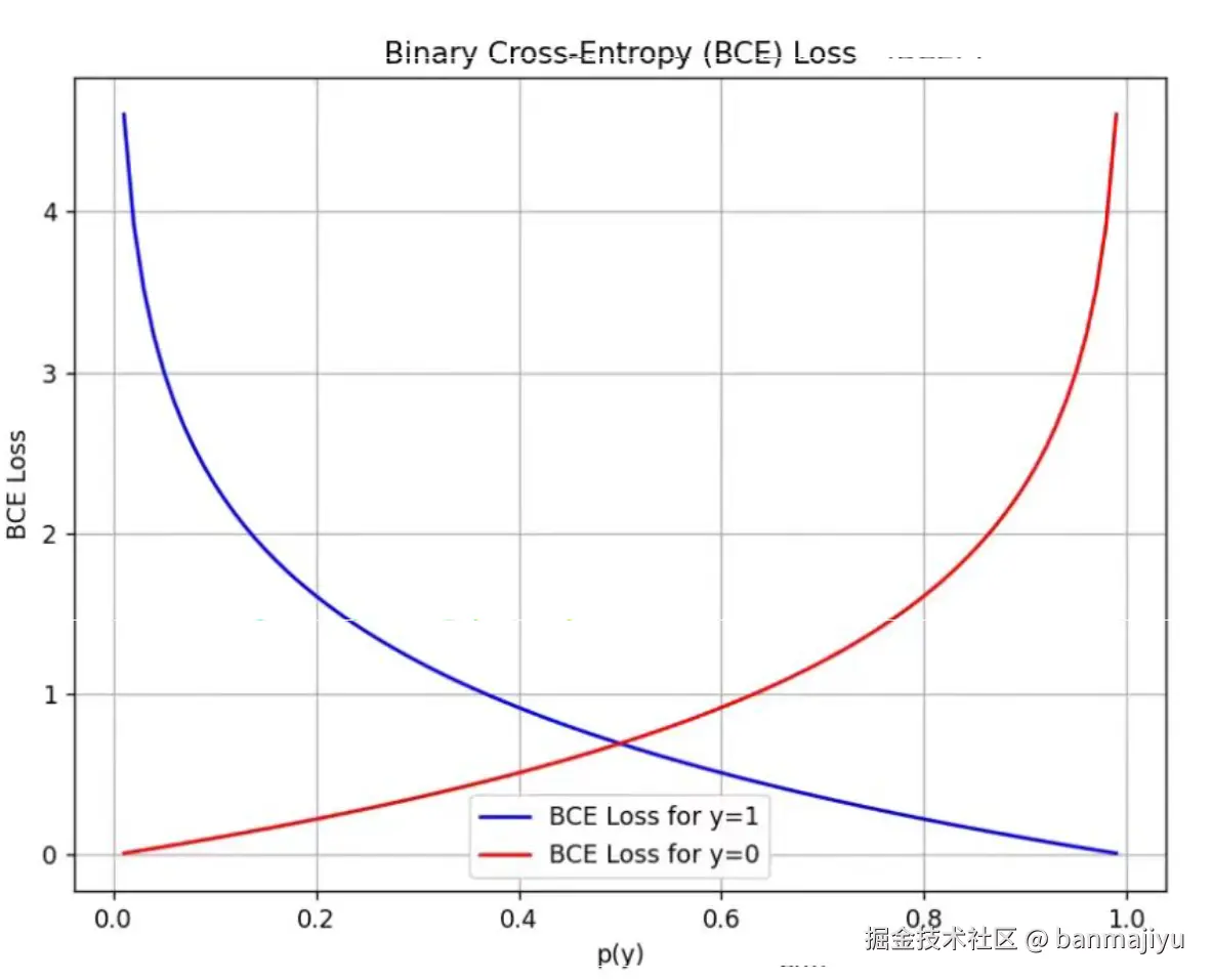
二元交叉熵：

<math xmlns="http://www.w3.org/1998/Math/MathML"> L = − [ y ⋅ log ⁡ ( y p r o b ) + ( 1 − y ) ⋅ log ⁡ ( 1 − y p r o b ) ] L=-[y\cdot\log(y_{prob})+(1-y)\cdot\log(1-y_{prob})] </math>L=−[y⋅log(yprob)+(1−y)⋅log(1−yprob)]

直观理解：

如果真实标签 <math xmlns="http://www.w3.org/1998/Math/MathML"> y = 1 y=1 </math>y=1，那么损失 <math xmlns="http://www.w3.org/1998/Math/MathML"> L = − log ⁡ ( y p r o b ) L=-\log(y_{prob}) </math>L=−log(yprob)。 <math xmlns="http://www.w3.org/1998/Math/MathML"> y p r o b y_{prob} </math>yprob越接近 <math xmlns="http://www.w3.org/1998/Math/MathML"> 1 1 </math>1，损失越小。
如果真实标签 <math xmlns="http://www.w3.org/1998/Math/MathML"> y = 0 y=0 </math>y=0，那么损失 <math xmlns="http://www.w3.org/1998/Math/MathML"> L = − log ⁡ ( 1 − y p r o b ) L=-\log(1-y_{prob}) </math>L=−log(1−yprob)。 <math xmlns="http://www.w3.org/1998/Math/MathML"> y p r o b y_{prob} </math>yprob越接近 <math xmlns="http://www.w3.org/1998/Math/MathML"> 1 1 </math>1，损失越大。

深度学习中的损失函数的统计学基础是极大似然估计 ，损失函数都是从最大似然估计开始推导的，不同数据分布会得出不同的损失函数。

二元交叉熵损失函数 ，本质上是二项分布下极大似然估计的负对数形式。它的目标是找到一组模型参数，使得我们观测到的样本数据同时出现的"可能性"最大。

给定观测数据 <math xmlns="http://www.w3.org/1998/Math/MathML"> D = { x 1 , x 2 , . . . , x n } D=\{x_1,x_2,...,x_n\} </math>D={x1,x2,...,xn}，我们要找到一个参数 <math xmlns="http://www.w3.org/1998/Math/MathML"> θ \theta </math>θ，使得所有观测数据同时出现的联合概率 <math xmlns="http://www.w3.org/1998/Math/MathML"> P ( D ∣ θ ) P(D|\theta) </math>P(D∣θ) 最大，这个 <math xmlns="http://www.w3.org/1998/Math/MathML"> θ \theta </math>θ 就是极大似然估计的估计值。PS：平常求概率的时候是不写参数的，因为参数（如硬币正面朝上的概率）是确定的，但这里参数是似然函数最终要求得的结果，所以这里就显式表明了参数的取值。

因为数据点通常独立同分布 ，联合概率等于每个数据点概率乘积：

<math xmlns="http://www.w3.org/1998/Math/MathML"> L ( θ ) = P ( D ∣ θ ) = ∏ i = 1 n P ( x i ∣ θ ) L(\theta)=P(D|\theta)=\prod \limits_{i=1}^n P(x_i|\theta) </math>L(θ)=P(D∣θ)=i=1∏nP(xi∣θ)

二分类问题中，样本的真实标签 <math xmlns="http://www.w3.org/1998/Math/MathML"> y y </math>y 的取值是 <math xmlns="http://www.w3.org/1998/Math/MathML"> 0 0 </math>0 或 <math xmlns="http://www.w3.org/1998/Math/MathML"> 1 1 </math>1，服从参数为 <math xmlns="http://www.w3.org/1998/Math/MathML"> p p </math>p 的二项分布：

<math xmlns="http://www.w3.org/1998/Math/MathML"> P ( Y = y ∣ p ) = p y ⋅ ( 1 − p ) 1 − y P(Y=y|p)=p^y\cdot(1-p)^{1-y} </math>P(Y=y∣p)=py⋅(1−p)1−y

也就是：

<math xmlns="http://www.w3.org/1998/Math/MathML"> P ( Y = 1 ∣ p ) = p , P ( Y = 0 ∣ p ) = 1 − p P(Y=1|p)=p, \space P(Y=0|p)=1-p </math>P(Y=1∣p)=p, P(Y=0∣p)=1−p

参数 <math xmlns="http://www.w3.org/1998/Math/MathML"> p p </math>p 是单层感知机的预测值 ，记作 <math xmlns="http://www.w3.org/1998/Math/MathML"> y ^ \hat y </math>y^。它是由输入 <math xmlns="http://www.w3.org/1998/Math/MathML"> x x </math>x 和参数 <math xmlns="http://www.w3.org/1998/Math/MathML"> θ \theta </math>θ 计算出来的，表示模型预测该样本的真实标签为 <math xmlns="http://www.w3.org/1998/Math/MathML"> 1 1 </math>1 的概率。

对于单个样本，其似然函数 表示样本数据在预测参数下发生的可能性，可以评判训练效果：

<math xmlns="http://www.w3.org/1998/Math/MathML"> L ( θ ∣ x , y ) = P ( Y = y ^ ) = y ^ y ⋅ ( 1 − y ^ ) 1 − y L(\theta|x,y)=P(Y=\hat{y})=\hat{y}^y\cdot(1-\hat{y})^{1-y} </math>L(θ∣x,y)=P(Y=y^)=y^y⋅(1−y^)1−y

对于 <math xmlns="http://www.w3.org/1998/Math/MathML"> n n </math>n 个独立样本，联合似然是每个样本似然的乘积，整个数据集的似然函数：

<math xmlns="http://www.w3.org/1998/Math/MathML"> L ( θ ) = ∏ i = 1 n y i ^ y i ⋅ ( 1 − y i ^ ) 1 − y i L(\theta)=\prod\limits_{i=1}^n \hat{y_i}^{y_i}\cdot(1-\hat{y_i})^{1-y_i} </math>L(θ)=i=1∏nyi^yi⋅(1−yi^)1−yi

乘积形式有诸多弊端，取对数，得到对数似然函数：

<math xmlns="http://www.w3.org/1998/Math/MathML"> log ⁡ ( L ( θ ) ) = ∑ i = 1 n [ y i ⋅ log ⁡ ( y i ^ ) + ( 1 − y i ) ⋅ log ⁡ ( 1 − y i ^ ) ] \log(L(\theta))=\sum\limits_{i=1}^n[y_i\cdot\log(\hat{y_i})+(1-y_i)\cdot\log(1-\hat{y_i})] </math>log(L(θ))=i=1∑n[yi⋅log(yi^)+(1−yi)⋅log(1−yi^)]

对数似然的相反数取平均值，得到二元交叉熵损失函数：

<math xmlns="http://www.w3.org/1998/Math/MathML"> L o s s ( θ ) = − 1 n log ⁡ ( L ( θ ) ) = − 1 n ∑ i = 1 n [ y i ⋅ log ⁡ ( y i ^ ) + ( 1 − y i ) ⋅ log ⁡ ( 1 − y i ^ ) ] Loss(\theta)=-\dfrac{1}{n}\log(L(\theta))=-\dfrac{1}{n}\sum\limits_{i=1}^n[y_i\cdot\log(\hat{y_i})+(1-y_i)\cdot\log(1-\hat{y_i})] </math>Loss(θ)=−n1log(L(θ))=−n1i=1∑n[yi⋅log(yi^)+(1−yi)⋅log(1−yi^)]

定义二元交叉熵为：

似然函数表示观测数据在当前模型预测参数下发生的可能性。模型预测得越准，似然函数越大，损失越小。

三、修改训练方式（梯度下降）

我们需要对损失函数求梯度，然后更新 <math xmlns="http://www.w3.org/1998/Math/MathML"> w \mathbf{w} </math>w和 <math xmlns="http://www.w3.org/1998/Math/MathML"> b b </math>b。

先求梯度：

<math xmlns="http://www.w3.org/1998/Math/MathML"> d L d y p r o b = − ( y y p r o b − 1 − y 1 − y p r o b ) \dfrac{\mathrm{d} L}{\mathrm{d} y_{prob}} = -(\dfrac{y}{y_{prob}}-\dfrac{1-y}{1-y_{prob}}) </math>dyprobdL=−(yproby−1−yprob1−y)

根据Sigmoid函数的定义：

<math xmlns="http://www.w3.org/1998/Math/MathML"> d y p r o b d z = y p r o b 1 − y p r o b , \dfrac{\mathrm{d} y_{prob}}{\mathrm{d} z} = \dfrac{y_{prob}}{1-y_{prob}}, </math>dzdyprob=1−yprobyprob, <math xmlns="http://www.w3.org/1998/Math/MathML"> d z d w = x , \dfrac{\mathrm{d} z}{\mathrm{d}w}=x, </math>dwdz=x, <math xmlns="http://www.w3.org/1998/Math/MathML"> d z d b = 1 \dfrac{\mathrm{d} z}{\mathrm{d}b}=1 </math>dbdz=1

根据链式法则：

<math xmlns="http://www.w3.org/1998/Math/MathML"> d L d z = d L d y p r o b ⋅ d y p r o b d z = y p r o b − y \dfrac{\mathrm{d} L}{\mathrm{d}z}= \dfrac{\mathrm{d} L}{\mathrm{d}y_{prob}} \cdot \dfrac{\mathrm{d} y_{prob}}{\mathrm{d}z}=y_{prob}-y </math>dzdL=dyprobdL⋅dzdyprob=yprob−y

同理，

<math xmlns="http://www.w3.org/1998/Math/MathML"> d L d w = ( y p r o b − y ) ⋅ x , \dfrac{\mathrm{d} L}{\mathrm{d}w}=(y_{prob}-y)\cdot x, </math>dwdL=(yprob−y)⋅x, <math xmlns="http://www.w3.org/1998/Math/MathML"> d L d b = y p r o b − y \dfrac{\mathrm{d} L}{\mathrm{d}b}=y_{prob}-y </math>dbdL=yprob−y

Sigmoid和二元交叉熵搭配，使得梯度恰好是(预测概率 - 真实标签)× 输入。

更新公式：

<math xmlns="http://www.w3.org/1998/Math/MathML"> w − = learning_rate × ( y p r o b − y ) × x w -= \text{learning\rate} \times (y{prob}-y)\times x </math>w−=learning_rate×(yprob−y)×x <math xmlns="http://www.w3.org/1998/Math/MathML"> b − = learning_rate × ( y p r o b − y ) b -= \text{learning\rate} \times (y{prob}-y) </math>b−=learning_rate×(yprob−y)

这和感知机更新很像，但是感知机是在分错时才更新 ，而逻辑回归是每步都更新。

四、完整代码

python 复制代码

import numpy as np

class LogisticRegression:
    def init(self, learning_rate=0.1, epochs=100):
        self.learning_rate = learning_rate  # 学习率
        self.epochs = epochs                # 迭代次数
        self.weights = None                 # 权重
        self.bias = None                    # 偏置

    def sigmoid(self, z):                   # Sigmoid函数
        return 1 / (1 + np.exp(-z))

    def fit(self, X, y):                    # 训练模型
        num_samples, num_features = X.shape # 样本数量和特征数量
        self.weights = np.zeros(num_features)   # 初始化权重
        self.bias = 0   # 初始化偏置

        for _ in range(self.epochs + 1):    # 迭代训练
            # 利用矩阵运算批量遍历样本
            linear_model = np.dot(X, self.weights) + self.bias  # 线性模型
            y_predicted = self.sigmoid(linear_model)    # 预测概率

            dw = (1 / num_samples) * np.dot(X.T, (y_predicted - y)) # 权重更新
            db = (1 / num_samples) * np.sum(y_predicted - y)    # 偏置更新

            self.weights -= self.learning_rate * dw # 更新权重
            self.bias -= self.learning_rate * db    # 更新偏置

            if _ % 100 == 0:  # 每100次迭代输出一次损失
                loss = -np.mean(y * np.log(y_predicted) + (1 - y) * np.log(1 - ypredicted))
                print(f'Epoch {}, Loss: {loss}, Weights: {self.weights}, Bias: {self.bias}, predicted: {y_predicted}')

    def predict(self, X):   # 预测新样本
        linear_model = np.dot(X, self.weights) + self.bias  # 线性模型
        y_predicted = self.sigmoid(linear_model)    # 预测概率
        y_predicted_cls = [i for i in y_predicted] # 分类结果
        return np.array(y_predicted_cls)    # 返回预测结果

我们用它来训练一个OR问题：

python 复制代码

# Example usage:
if name == "main":
    # dataset
    X = np.array([[0, 0],
                  [0, 1],
                  [1, 0],
                  [1, 1]])
    y = np.array([0, 1, 1, 1])  # labels

    model = LogisticRegression(epochs=1000, learning_rate=0.1)
    model.fit(X, y)
    predictions = model.predict(X)
    print("Predictions:", predictions)

输出结果：

python 复制代码

Epoch 0, Loss: 0.6931471805599453, Weights: [0.025 0.025], Bias: 0.025, predicted: [0.5 0.5 0.5 0.5]
Epoch 100, Loss: 0.3422648179240876, Weights: [1.12179346 1.12179346], Bias: 0.3241873928250224, predicted: [0.58111698 0.80885348 0.80885348 0.92809543]
Epoch 200, Loss: 0.2668907776248633, Weights: [1.67965174 1.67965174], Bias: -0.028037186370862888, predicted: [0.49384689 0.83891033 0.83891033 0.96527318]
Epoch 300, Loss: 0.21739481429264515, Weights: [2.12500033 2.12500033], Bias: -0.336940396505239, predicted: [0.41722497 0.85652781 0.85652781 0.98030824]
Epoch 400, Loss: 0.18253957593342224, Weights: [2.50261016 2.50261016], Bias: -0.585446486877449, predicted: [0.35819515 0.8716802  0.8716802  0.98804998]
Epoch 500, Loss: 0.15679759961756431, Weights: [2.83028441 2.83028441], Bias: -0.7896551756986915, predicted: [0.31264419 0.88487511 0.88487511 0.99235967]
Epoch 600, Loss: 0.1370743652412334, Weights: [3.11907017 3.11907017], Bias: -0.962306596435656, predicted: [0.27673684 0.89619475 0.89619475 0.99489283]
Epoch 700, Loss: 0.1215219182866978, Weights: [3.37672399 3.37672399], Bias: -1.1117282082003561, predicted: [0.24780951 0.90584725 0.90584725 0.99645347]
Epoch 800, Loss: 0.1089723627417807, Weights: [3.60894888 3.60894888], Bias: -1.2433997965996983, predicted: [0.22406065 0.91408616 0.91408616 0.99745561]
Epoch 900, Loss: 0.09865242980397079, Weights: [3.82005709 3.82005709], Bias: -1.3610689169623034, predicted: [0.20424809 0.92115082 0.92115082 0.99812286]
Epoch 1000, Loss: 0.09003038954892699, Weights: [4.01338124 4.01338124], Bias: -1.4674033054431226, predicted: [0.18749206 0.92724619 0.92724619 0.9985814 ]
Predictions: [0.18733762 0.92730284 0.92730284 0.99858521]

训练AND问题：

python 复制代码

# Example usage:
if name == "main":
    # dataset
    X = np.array([[0, 0],
                  [0, 1],
                  [1, 0],
                  [1, 1]])
    y = np.array([0, 0, 0, 1])  # labels

    model = LogisticRegression(epochs=1000, learningrate=0.1)
    model.fit(X, y)
    predictions = model.predict(X)
    print("Predictions:", predictions)

输出结果：

python 复制代码

Epoch 0, Loss: 0.6931471805599453, Weights: [0. 0.], Bias: -0.025, predicted: [0.5 0.5 0.5 0.5]
Epoch 100, Loss: 0.46240131259227135, Weights: [0.51290945 0.51290945], Bias: -1.2534222714262722, predicted: [0.22346095 0.32331948 0.32331948 0.44238052]
Epoch 200, Loss: 0.3632692335353307, Weights: [1.02689924 1.02689924], Bias: -1.926427902775465, predicted: [0.12780757 0.28944671 0.28944671 0.53104471]
Epoch 300, Loss: 0.3018586895621536, Weights: [1.42642895 1.42642895], Bias: -2.4656161027608676, predicted: [0.07866    0.26156517 0.26156517 0.59507742]
Epoch 400, Loss: 0.25956392625978153, Weights: [1.75358999 1.75358999], Bias: -2.9204394490304124, predicted: [0.05135764 0.23764547 0.23764547 0.64220664]
Epoch 500, Loss: 0.22828521633076554, Weights: [2.03250361 2.03250361], Bias: -3.3154992464345603, predicted: [0.03516893 0.2172292  0.2172292  0.67874626]
Epoch 600, Loss: 0.20400582757628868, Weights: [2.27681838 2.27681838], Bias: -3.6658032435287673, predicted: [0.02502622 0.19973196 0.19973196 0.7081768 ]
Epoch 700, Loss: 0.1845024840587356, Weights: [2.4949078 2.4949078], Bias: -3.981140706476398, predicted: [0.01837648 0.1846283  0.1846283  0.73253796]
Epoch 800, Loss: 0.1684341099874634, Weights: [2.69228575 2.69228575], Bias: -4.268256220819802, predicted: [0.01385021 0.1714896  0.1714896  0.75311478]
Epoch 900, Loss: 0.1549360688551386, Weights: [2.87279509 2.87279509], Bias: -4.532013815281678, predicted: [0.01067119 0.15997482 0.15997482 0.77076718]
Epoch 1000, Loss: 0.1434211628893327, Weights: [3.03923779 3.03923779], Bias: -4.776054827817194, predicted: [0.00837825 0.14981323 0.14981323 0.78609892]
Predictions: [0.00835873 0.14971768 0.14971768 0.78624211]

五、调整

训练轮数

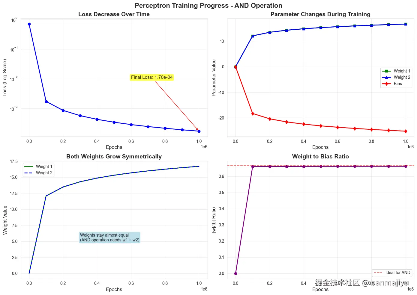
以AND问题为例，将训练轮数改为 <math xmlns="http://www.w3.org/1998/Math/MathML"> 1000000 1000000 </math>1000000轮，每 <math xmlns="http://www.w3.org/1998/Math/MathML"> 100000 100000 </math>100000轮训练输出一次结果，如下：

python 复制代码

Epoch 0, Loss: 0.6931471805599453, Weights: [0. 0.], Bias: -0.025, predicted: [0.5 0.5 0.5 0.5]
Epoch 100000, Loss: 0.0017135254130423991, Weights: [12.07442273 12.07442273], Bias: -18.28028667121314, predicted: [1.15076192e-08 2.01352286e-03 2.01352286e-03 9.97180996e-01]
Epoch 200000, Loss: 0.0008540609215053913, Weights: [13.46827331 13.46827331], Bias: -20.370853295163833, predicted: [1.42251667e-09 1.00418435e-03 1.00418435e-03 9.98594125e-01]
Epoch 300000, Loss: 0.0005686482917795434, Weights: [14.28216591 14.28216591], Bias: -21.59162287967754, predicted: [4.19644644e-10 6.68735073e-04 6.68735073e-04 9.99063763e-01]
Epoch 400000, Loss: 0.00042618526123873744, Weights: [14.85914749 14.85914749], Bias: -22.457060672544646, predicted: [1.76614248e-10 5.01246758e-04 5.01246758e-04 9.99298250e-01]
Epoch 500000, Loss: 0.00034079363305620255, Weights: [15.30646479 15.30646479], Bias: -23.128015908723395, predicted: [9.02886012e-11 4.00839271e-04 4.00839271e-04 9.99438822e-01]
Epoch 600000, Loss: 0.0002839043730732245, Weights: [15.6718262 15.6718262], Bias: -23.676044225842773, predicted: [5.21947492e-11 3.33939623e-04 3.33939623e-04 9.99532483e-01]
Epoch 700000, Loss: 0.00024328905189608215, Weights: [15.98065927 15.98065927], Bias: -24.139283972824206, predicted: [3.28430921e-11 2.86174300e-04 2.86174300e-04 9.99599355e-01]
Epoch 800000, Loss: 0.0002128388867211385, Weights: [16.24813277 16.24813277], Bias: -24.540486841549885, predicted: [2.19889055e-11 2.50361867e-04 2.50361867e-04 9.99649492e-01]
Epoch 900000, Loss: 0.0001891623721345687, Weights: [16.48402639 16.48402639], Bias: -24.894321536210516, predicted: [1.54360073e-11 2.22514882e-04 2.22514882e-04 9.99688478e-01]
Epoch 1000000, Loss: 0.00017022566760183658, Weights: [16.69501522 16.69501522], Bias: -25.210800188506223, predicted: [1.12483779e-11 2.00241938e-04 2.00241938e-04 9.99719661e-01]
Predictions: [1.12483441e-11 2.00241738e-04 2.00241738e-04 9.99719661e-01]

训练用时 <math xmlns="http://www.w3.org/1998/Math/MathML"> 7.3 7.3 </math>7.3秒，详细分析如下：

模型收敛
- 损失函数持续下降 ：损失（Loss）从初始的约 <math xmlns="http://www.w3.org/1998/Math/MathML"> 0.693 0.693 </math>0.693稳定下降至 <math xmlns="http://www.w3.org/1998/Math/MathML"> 0.00017 0.00017 </math>0.00017，表明梯度下降算法工作正常，模型参数在不断优化。
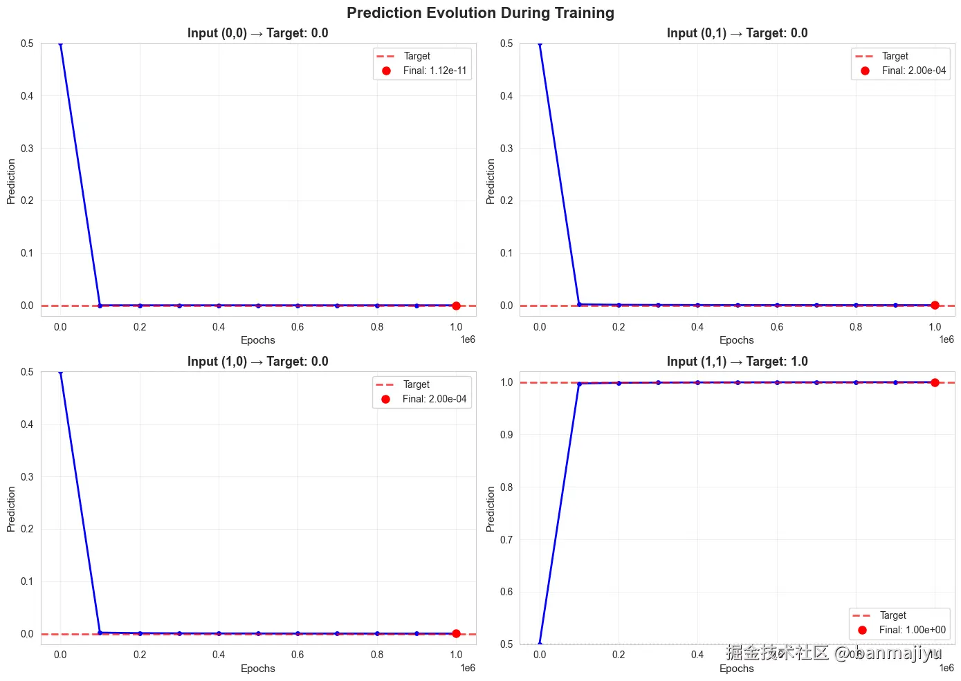
- 预测值逼近理论值 ：最终的预测结果 <math xmlns="http://www.w3.org/1998/Math/MathML"> [ ≈ 0 , 0.0002 , 0.0002 , 0.9997 ] [\approx 0, 0.0002, 0.0002, 0.9997] </math>[≈0,0.0002,0.0002,0.9997]，几乎等同于AND运算的真值表 <math xmlns="http://www.w3.org/1998/Math/MathML"> [ 0 , 0 , 0 , 1 ] [0, 0, 0, 1] </math>[0,0,0,1]。
参数演变
- 权重对称增长 ：两个权重（Weights）在训练中始终保持相等，最终都约为 <math xmlns="http://www.w3.org/1998/Math/MathML"> 16.70 16.70 </math>16.70。这完全合理，因为对于AND运算，两个输入特征（ <math xmlns="http://www.w3.org/1998/Math/MathML"> x 1 x_1 </math>x1和 <math xmlns="http://www.w3.org/1998/Math/MathML"> x 2 x_2 </math>x2）具有同等重要性。
- 偏置大幅负向调整 ：偏置（Bias）从 <math xmlns="http://www.w3.org/1998/Math/MathML"> − 0.025 -0.025 </math>−0.025变为 <math xmlns="http://www.w3.org/1998/Math/MathML"> − 25.21 -25.21 </math>−25.21。这个很大的负值帮助模型在输入为 <math xmlns="http://www.w3.org/1998/Math/MathML"> ( 0 , 0 ) , ( 0 , 1 ) , ( 1 , 0 ) (0,0), (0,1), (1,0) </math>(0,0),(0,1),(1,0)时，将加权和压制到负数区间，使得sigmoid输出接近 <math xmlns="http://www.w3.org/1998/Math/MathML"> 0 0 </math>0。
训练过程
- 初期（Epoch <math xmlns="http://www.w3.org/1998/Math/MathML"> 0 0 </math>0）：参数初始化为 <math xmlns="http://www.w3.org/1998/Math/MathML"> 0 0 </math>0附近，输出均为 <math xmlns="http://www.w3.org/1998/Math/MathML"> 0.5 0.5 </math>0.5，相当于随机猜测。
- 中期（如Epoch <math xmlns="http://www.w3.org/1998/Math/MathML"> 100 k 100k </math>100k）：损失迅速下降，预测值开始显现AND逻辑的轮廓。
- 后期（Epoch <math xmlns="http://www.w3.org/1998/Math/MathML"> 500 k → 1 M 500k \to 1M </math>500k→1M）：损失下降速度变缓，进入微调阶段。模型持续增大权重和偏置的绝对值，以驱使sigmoid函数的输出无限接近 <math xmlns="http://www.w3.org/1998/Math/MathML"> 0 0 </math>0或 <math xmlns="http://www.w3.org/1998/Math/MathML"> 1 1 </math>1，从而进一步减小损失。

可视化：

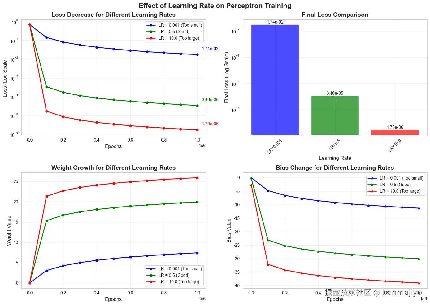
学习率

在刚刚训练的基础上，调整学习率为 <math xmlns="http://www.w3.org/1998/Math/MathML"> 0.001 0.001 </math>0.001、 <math xmlns="http://www.w3.org/1998/Math/MathML"> 0.5 0.5 </math>0.5、 <math xmlns="http://www.w3.org/1998/Math/MathML"> 10.0 10.0 </math>10.0，结果如下：

python 复制代码

===Learning rate: 0.001===
Epoch 0, Loss: 0.6931471805599453, Weights: [0. 0.], Bias: -0.00025, predicted: [0.5 0.5 0.5 0.5]
Epoch 100000, Loss: 0.14350630119487667, Weights: [3.03637282 3.03637282], Bias: -4.77184972987911, predicted: [0.00839385 0.14988932 0.14988932 0.78598429]
Epoch 200000, Loss: 0.08166141124133444, Weights: [4.2367081 4.2367081], Bias: -6.547040329576306, predicted: [0.00143232 0.09027123 0.09027123 0.87284722]
Epoch 300000, Loss: 0.056559316473414695, Weights: [5.00411178 5.00411178], Bias: -7.689883791945169, predicted: [4.57226574e-04 6.38183450e-02 6.38183450e-02 9.10384315e-01]
Epoch 400000, Loss: 0.04307253011634129, Weights: [5.56721754 5.56721754], Bias: -8.530492084519793, predicted: [1.97320344e-04 4.91129704e-02 4.91129704e-02 9.31114753e-01]
Epoch 500000, Loss: 0.034699854291060435, Weights: [6.01108681 6.01108681], Bias: -9.193904140467376, predicted: [1.01647480e-04 3.98175578e-02 3.98175578e-02 9.44184367e-01]
Epoch 600000, Loss: 0.029014140880282528, Weights: [6.37693375 6.37693375], Bias: -9.741100438933035, predicted: [5.88126121e-05 3.34343625e-02 3.34343625e-02 9.53147504e-01]
Epoch 700000, Loss: 0.024908812646655665, Weights: [6.68783334 6.68783334], Bias: -10.206337367707393, predicted: [3.69342969e-05 2.87903360e-02 2.87903360e-02 9.59663574e-01]
Epoch 800000, Loss: 0.02180930061451368, Weights: [6.9579869 6.9579869], Bias: -10.610740793726809, predicted: [2.46493099e-05 2.52648267e-02 2.52648267e-02 9.64607854e-01]
Epoch 900000, Loss: 0.019388415347494817, Weights: [7.19674494 7.19674494], Bias: -10.968239590717861, predicted: [1.72404282e-05 2.24997681e-02 2.24997681e-02 9.68484383e-01]
Epoch 1000000, Loss: 0.01744648186578177, Weights: [7.41058505 7.41058505], Bias: -11.28849247685743, predicted: [1.25160098e-05 2.02745412e-02 2.02745412e-02 9.71603354e-01]
Predictions: [1.25159717e-05 2.02745211e-02 2.02745211e-02 9.71603382e-01]
===Learning rate: 0.5===
Epoch 0, Loss: 0.6931471805599453, Weights: [0. 0.], Bias: -0.125, predicted: [0.5 0.5 0.5 0.5]
Epoch 100000, Loss: 0.00034078325774289646, Weights: [15.30654173 15.30654173], Bias: -23.128131313111425, predicted: [9.02803532e-11 4.00827071e-04 4.00827071e-04 9.99438839e-01]
Epoch 200000, Loss: 0.00017022284180639367, Weights: [16.69505643 16.69505643], Bias: -25.21086200947468, predicted: [1.12478177e-11 2.00238614e-04 2.00238614e-04 9.99719665e-01]
Epoch 300000, Loss: 0.00011343940872846477, Weights: [17.50681486 17.50681486], Bias: -26.428485898148118, predicted: [3.32857813e-12 1.33447668e-04 1.33447668e-04 9.99813173e-01]
Epoch 400000, Loss: 8.506247665863291e-05, Weights: [18.08262019 18.08262019], Bias: -27.292187009328256, predicted: [1.40332106e-12 1.00067621e-04 1.00067621e-04 9.99859905e-01]
Epoch 500000, Loss: 6.804138020102558e-05, Weights: [18.52918387 18.52918387], Bias: -27.962028408320233, predicted: [7.18204243e-13 8.00449198e-05 8.00449198e-05 9.99887937e-01]
Epoch 600000, Loss: 5.6696194752500084e-05, Weights: [18.89401763 18.89401763], Bias: -28.50927629810481, predicted: [4.15509343e-13 6.66987930e-05 6.66987930e-05 9.99906622e-01]
Epoch 700000, Loss: 4.859361465153441e-05, Weights: [19.20245887 19.20245887], Bias: -28.97193619207216, predicted: [2.61607291e-13 5.71670392e-05 5.71670392e-05 9.99919966e-01]
Epoch 800000, Loss: 4.251731256003311e-05, Weights: [19.46962893 19.46962893], Bias: -29.372689818942614, predicted: [1.75228411e-13 5.00188985e-05 5.00188985e-05 9.99929974e-01]
Epoch 900000, Loss: 3.779168431031443e-05, Weights: [19.70528006 19.70528006], Bias: -29.72616535772023, predicted: [1.23052903e-13 4.44596443e-05 4.44596443e-05 9.99937756e-01]
Epoch 1000000, Loss: 3.401142913063264e-05, Weights: [19.91607027 19.91607027], Bias: -30.042349765450773, predicted: [8.96963099e-14 4.00125059e-05 4.00125059e-05 9.99943982e-01]
Predictions: [8.96960408e-14 4.00124658e-05 4.00124658e-05 9.99943983e-01]
===Learning rate: 10.0===
Epoch 0, Loss: 0.6931471805599453, Weights: [0. 0.], Bias: -2.5, predicted: [0.5 0.5 0.5 0.5]
Epoch 100000, Loss: 1.700081895673019e-05, Weights: [21.30298324 21.30298324], Bias: -32.12271509481572, predicted: [1.12019884e-14 2.00007286e-05 2.00007286e-05 9.99971999e-01]
Epoch 200000, Loss: 8.500258629958978e-06, Weights: [22.68931547 22.68931547], Bias: -34.202211376766336, predicted: [1.40015090e-15 1.00002455e-05 1.00002455e-05 9.99986000e-01]
Epoch 300000, Loss: 5.666795624017699e-06, Weights: [23.50026181 23.50026181], Bias: -35.4186302107126, predicted: [4.14847699e-16 6.66679228e-06 6.66679228e-06 9.99990666e-01]
Epoch 400000, Loss: 4.25007813009538e-06, Weights: [24.0756351 24.0756351], Bias: -36.28168979891588, predicted: [1.75011096e-16 5.00007724e-06 5.00007724e-06 9.99993000e-01]
Epoch 500000, Loss: 3.400052779115479e-06, Weights: [24.52192816 24.52192816], Bias: -36.95112918376485, predicted: [8.96047642e-17 4.00005270e-06 4.00005270e-06 9.99994400e-01]
Epoch 600000, Loss: 2.8333715605258275e-06, Weights: [24.8865755 24.8865755], Bias: -37.49810004814846, predicted: [5.18542359e-17 3.33337178e-06 3.33337178e-06 9.99995333e-01]
Epoch 700000, Loss: 2.4286004922126167e-06, Weights: [25.19488002 25.19488002], Bias: -37.96055673278328, predicted: [3.26543875e-17 2.85717226e-06 2.85717226e-06 9.99996000e-01]
Epoch 800000, Loss: 2.1250229006839423e-06, Weights: [25.46194527 25.46194527], Bias: -38.36115453597536, predicted: [2.18757975e-17 2.50002327e-06 2.50002327e-06 9.99996500e-01]
Epoch 900000, Loss: 1.8889074354947174e-06, Weights: [25.69751332 25.69751332], Bias: -38.714506558669086, predicted: [1.53640206e-17 2.22224114e-06 2.22224114e-06 9.99996889e-01]
Epoch 1000000, Loss: 1.7000153503880637e-06, Weights: [25.90823598 25.90823598], Bias: -39.030590506399825, predicted: [1.12003404e-17 2.00001571e-06 2.00001571e-06 9.99997200e-01]
Predictions: [1.12003068e-17 2.00001371e-06 2.00001371e-06 9.99997200e-01]

训练用时 <math xmlns="http://www.w3.org/1998/Math/MathML"> 22.0 22.0 </math>22.0秒

核心结论

学习率是控制训练速度与稳定性的关键超参数。对于此AND运算任务：

学习率 <math xmlns="http://www.w3.org/1998/Math/MathML"> = 0.001 =0.001 </math>=0.001：过小，导致收敛极其缓慢，未能充分学习。
学习率 <math xmlns="http://www.w3.org/1998/Math/MathML"> = 0.5 =0.5 </math>=0.5：适中，收敛稳健有效，比之前 <math xmlns="http://www.w3.org/1998/Math/MathML"> 0.1 0.1 </math>0.1的表现还要好。
学习率 <math xmlns="http://www.w3.org/1998/Math/MathML"> = 10.0 =10.0 </math>=10.0：偏大，收敛速度最快，但带来了数值风险。

详细对比分析

分析维度	学习率 = <math xmlns="http://www.w3.org/1998/Math/MathML"> 0.001 0.001 </math>0.001 (过小)	学习率 = <math xmlns="http://www.w3.org/1998/Math/MathML"> 0.5 0.5 </math>0.5 (适中)	学习率 = <math xmlns="http://www.w3.org/1998/Math/MathML"> 10.0 10.0 </math>10.0 (偏大)	对比与解读
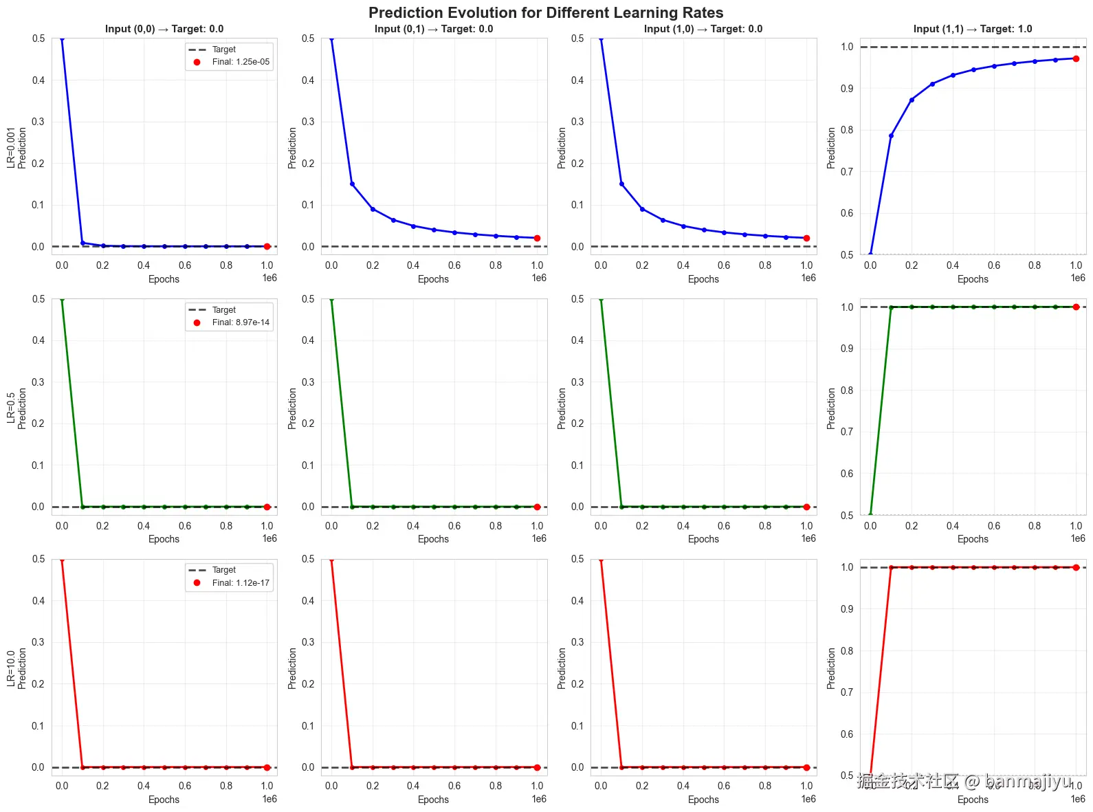
1. 模型收敛	收敛不足。100万轮后`Loss`仍高达 <math xmlns="http://www.w3.org/1998/Math/MathML"> 0.017 0.017 </math>0.017，预测值( <math xmlns="http://www.w3.org/1998/Math/MathML"> [ 0.00001 , 0.0203 , 0.0203 , 0.9716 ] [0.00001, 0.0203, 0.0203, 0.9716] </math>[0.00001,0.0203,0.0203,0.9716])远未逼近理论值( <math xmlns="http://www.w3.org/1998/Math/MathML"> [ 0 , 0 , 0 , 1 ] [0,0,0,1] </math>[0,0,0,1])。	收敛良好。`Loss`稳步降至3.4e-5，预测值([~0, 0.00004, 0.00004, 0.99994])已极度接近理论值。	收敛最快。`Loss`降至1.7e-6（为0.5时的1/20），预测值最接近理论值。	学习率越大，单次参数更新步长越大，收敛至低`Loss`的速度越快。但 <math xmlns="http://www.w3.org/1998/Math/MathML"> 0.001 0.001 </math>0.001的步长太小，参数更新"力气不足"，无法有效逼近最优解。
2. 参数演变	参数增长缓慢：权重≈ <math xmlns="http://www.w3.org/1998/Math/MathML"> 7.41 7.41 </math>7.41，偏置≈ <math xmlns="http://www.w3.org/1998/Math/MathML"> − 11.29 -11.29 </math>−11.29。绝对值较小，无法将`sigmoid`输出"推"向 <math xmlns="http://www.w3.org/1998/Math/MathML"> 0 0 </math>0或 <math xmlns="http://www.w3.org/1998/Math/MathML"> 1 1 </math>1的极端。	参数增长稳健：权重≈ <math xmlns="http://www.w3.org/1998/Math/MathML"> 19.92 19.92 </math>19.92，偏置≈ <math xmlns="http://www.w3.org/1998/Math/MathML"> − 30.04 -30.04 </math>−30.04。通过持续调整，有效驱动了`sigmoid`的输出。	参数增长极大：权重≈ <math xmlns="http://www.w3.org/1998/Math/MathML"> 25.91 25.91 </math>25.91，偏置≈ <math xmlns="http://www.w3.org/1998/Math/MathML"> − 39.03 -39.03 </math>−39.03。数值最大，这是用更大更新步长快速逼近最优解的副作用。	所有情况下权重始终保持对称（ <math xmlns="http://www.w3.org/1998/Math/MathML"> W 1 = W 2 W_1=W_2 </math>W1=W2），完美体现了`AND`运算中两个输入权值相等的特性。学习率越大，最终参数的绝对值越大。
3. 训练过程	损失曲线下降平缓，效率低下。需要远超 <math xmlns="http://www.w3.org/1998/Math/MathML"> 100 100 </math>100万轮的迭代才可能达到其他学习率的效果。	损失曲线平滑、稳定下降，是理想的学习过程。与之前学习率 <math xmlns="http://www.w3.org/1998/Math/MathML"> 0.1 0.1 </math>0.1的轨迹高度相似，只是步长稍大。	损失初期下降迅猛。但存在潜在风险：如此大的学习率在更复杂模型或数据上极易导致`Loss`震荡（来回跳跃）甚至发散，此处因问题简单而未显现。	展示了学习率作为"步幅"的核心作用：小步稳但慢，大步快但险。

可视化：

激活函数

我们想看看不同激活函数对训练的影响 ，但是每次修改激活函数都需要重新求导 <math xmlns="http://www.w3.org/1998/Math/MathML"> + + </math>+ 修改代码。利用模块化的思想，我们定义一个Activation类，它包含向前（原函数）和向后（导数）两部分。求导这一块可以丢给Vibe Coding：）
其次，交叉熵损失函数只适配Sigmoid函数，所以我们采用更通用的MSE损失函数。

MSE

均方误差 （Mean Squared Error），也称为L2损失。它是机器学习中最常用的回归任务损失函数 之一，用于衡量模型预测值与真实值之间的差异。

1. 数学定义

对于一个有 <math xmlns="http://www.w3.org/1998/Math/MathML"> m m </math>m个样本的数据集：

<math xmlns="http://www.w3.org/1998/Math/MathML"> M S E = 1 m ∑ i = 1 m ( y i − y ^ i ) 2 \mathrm{MSE} = \dfrac{1}{m} \sum \limits_{i=1}^m(y_i-\hat y_i)^2 </math>MSE=m1i=1∑m(yi−y^i)2

<math xmlns="http://www.w3.org/1998/Math/MathML"> y i y_i </math>yi：第 <math xmlns="http://www.w3.org/1998/Math/MathML"> i i </math>i 个样本的真实值
<math xmlns="http://www.w3.org/1998/Math/MathML"> y ^ i \hat y_i </math>y^i：第 <math xmlns="http://www.w3.org/1998/Math/MathML"> i i </math>i个样本的预测值
公式先计算每个样本的预测误差（残差），然后平方（使误差为正且放大较大误差），最后对所有样本取平均。

2. 直观理解

目标：MSE的值越小越好，完美预测时MSE为0。
特点：由于平方项，MSE对较大的误差（离群点）惩罚更重，这使得模型对异常值比较敏感。
可视化：它是一个平滑的、凸的抛物线形函数，有利于梯度下降等优化算法找到最小值。

3. 对比

之前的代码使用的是交叉熵损失 （Cross-Entropy Loss），它适用于分类问题（输出解释为概率）。而MSE是一种通用的损失函数。

对比维度	交叉熵损失	均方误差（MSE）
主要用途	分类（特别是二分类、多分类	回归（预测连续值）
输出要求	预测值必须在 <math xmlns="http://www.w3.org/1998/Math/MathML"> ( 0 , 1 ) (0, 1) </math>(0,1)之间（如`Sigmoid`输出）	预测值可以是任意实数（无范围限制）
梯度特性	与`Sigmoid`结合时梯度简洁 <math xmlns="http://www.w3.org/1998/Math/MathML"> ( y p r e d − y ) (y_{pred} - y) </math>(ypred−y)	梯度形式简单通用 <math xmlns="http://www.w3.org/1998/Math/MathML"> ( y p r e d − y ) (y_{pred} - y) </math>(ypred−y)
在代码中的问题	若激活函数输出不在 <math xmlns="http://www.w3.org/1998/Math/MathML"> ( 0 , 1 ) (0,1) </math>(0,1)内（如`ReLU`负数、`Tanh`负值），`log`计算会出`NaN`	对任何输出值都有效，不会因`log`计算而崩溃

4. 梯度公式

使用MSE时，损失函数对于第 <math xmlns="http://www.w3.org/1998/Math/MathML"> i i </math>i 个样本的梯度为：

<math xmlns="http://www.w3.org/1998/Math/MathML"> ∂ M S E ∂ y ^ i = 2 ( y i − y ^ i ) \dfrac{\partial MSE}{\partial \hat y_i}=2(y_i-\hat y_i) </math>∂y^i∂MSE=2(yi−y^i)

在实际的梯度下降中，常数因子 <math xmlns="http://www.w3.org/1998/Math/MathML"> 2 2 </math>2 通常被吸收到学习率中，因此简化为：

<math xmlns="http://www.w3.org/1998/Math/MathML"> y i − y ^ i y_i-\hat y_i </math>yi−y^i

完整梯度：

<math xmlns="http://www.w3.org/1998/Math/MathML"> ∂ L o s s ∂ w j = 1 m ( ∑ i = 1 m ( y i − y ^ i ) ) ⋅ ∂ y ^ i ∂ z i ⋅ x i j \dfrac{\partial Loss}{\partial w_j} = \dfrac{1}{m}(\sum\limits_{i=1}^m(y_i-\hat y_i))\cdot\dfrac{\partial\hat y_i}{\partial z_i}\cdot x_{ij} </math>∂wj∂Loss=m1(i=1∑m(yi−y^i))⋅∂zi∂y^i⋅xij <math xmlns="http://www.w3.org/1998/Math/MathML"> ∂ L o s s ∂ b = 1 m ( ∑ i = 1 m ( y i − y ^ i ) ) ⋅ ∂ y ^ i ∂ z i \dfrac{\partial Loss}{\partial b} = \dfrac{1}{m}(\sum\limits_{i=1}^m(y_i-\hat y_i))\cdot\dfrac{\partial\hat y_i}{\partial z_i} </math>∂b∂Loss=m1(i=1∑m(yi−y^i))⋅∂zi∂y^i

其中 <math xmlns="http://www.w3.org/1998/Math/MathML"> ∂ y ^ i ∂ z i \dfrac{\partial\hat y_i}{\partial z_i} </math>∂zi∂y^i就是activation.backward(linear_model)。

总结

所以，如果想快速测试不同激活函数是否"能学"，换成MSE是一个简单有效的调试策略 。但要获得最好的分类性能，对于二分类任务，Sigmoid + 交叉熵仍然是标准组合。

代码实现：

python 复制代码

import numpy as np

class Activation:
    def forward(self, x):   # 前向传播
        raise NotImplementedError
    
    def backward(self, x):  # 反向传播
        raise NotImplementedError
    
# === 一大堆激活函数 ===

class Sigmoid(Activation):  # Sigmoid激活函数
    def forward(self, x):
        return 1 / (1 + np.exp(-x))
    
    def backward(self, x):
        s = self.forward(x)
        return s * (1 - s)
    
class ReLU(Activation): # ReLU激活函数
    def forward(self, x):
        return np.maximum(0, x)
    
    def backward(self, x):
        return np.where(x > 0, 1, 0)
    
class Tanh(Activation): # Tanh激活函数
    def forward(self, x):
        return np.tanh(x)
    
    def backward(self, x):
        t = self.forward(x)
        return 1 - t ** 2
    
class LeakyReLU(Activation):    # Leaky ReLU激活函数
    def init(self, alpha=0.01):
        self.alpha = alpha
    
    def forward(self, x):
        return np.where(x > 0, x, self.alpha * x)
    
    def backward(self, x):
        return np.where(x > 0, 1, self.alpha)
    
class Cube(Activation):  # Cube激活函数
    def forward(self, x):
        return x ** 3
    
    def backward(self, x):
        return 3 * x ** 2
    
class Arctan(Activation):    # Arctan激活函数
    def forward(self, x):
        return np.arctan(x)
    
    def backward(self, x):
        return 1 / (1 + x ** 2)
    
class Sine(Activation):  # Sine激活函数
    def forward(self, x):
        return np.sin(x)
    
    def backward(self, x):
        return np.cos(x)
    
class Step(Activation):  # Step激活函数
    def forward(self, x):
        return np.where(x >= 0, 1, 0)
    
    def backward(self, x):
        return np.zeros_like(x)
    
class Square(Activation):    # Square激活函数
    def forward(self, x):
        return x ** 2
    
    def backward(self, x):
        return 2 * x
    
class Random(Activation):    # Random激活函数
    def forward(self, x):
        return np.random.rand(*x.shape)
    
    def backward(self, x):
        return np.zeros_like(x)

class LogisticRegression:
    def init(self, learning_rate=0.1, epochs=100, activation=Sigmoid()):
        self.learning_rate = learning_rate
        self.epochs = epochs
        self.activation = activation
        self.weights = None
        self.bias = None

    # 修改fit方法如下：
    def fit(self, X, y):
        num_samples, num_features = X.shape
        self.weights = np.random.randn(num_features) * 0.01    #初始值优化
        self.bias = 0.0

        for epoch in range(self.epochs + 1):
            linear_model = np.dot(X, self.weights) + self.bias
            y_predicted = self.activation.forward(linear_model)
            error = y_predicted - y # 计算MSE误差
        
            grad_activation = self.activation.backward(linear_model)    # 激活函数的梯度
            dL_dz = error * grad_activation  # 链式法则
        
            dw = (1 / num_samples) * np.dot(X.T, dL_dz) # 权重的梯度
            db = (1 / num_samples) * np.sum(dL_dz)      # 偏置的梯度
        
            self.weights -= self.learning_rate * dw     # 更新权重
            self.bias -= self.learning_rate * db        # 更新偏置
        
            if epoch % (self.epochs // 10) == 0:        # 输出损失
                loss = np.mean(error ** 2)
                print(f'Epoch {epoch}, Loss: {loss}, Weights: {self.weights}, Bias: {self.bias}, predicted: {y_predicted}')


    def predict(self, X):
        linear_model = np.dot(X, self.weights) + self.bias
        y_predicted = self.activation.forward(linear_model)
        y_predicted_cls = [i for i in y_predicted]
        return np.array(y_predicted_cls)
    
# Example usage AND :
if name == "main":
    X = np.array([[0, 0],
                  [0, 1],
                  [1, 0],
                  [1, 1]])
    y = np.array([0, 0, 0, 1])  # labels

    activates = [Sigmoid(), ReLU(), Tanh(), LeakyReLU(), Cube(), Arctan(), Sine(), Step(), Square(), Random()]  # 不同的激活函数
    for activate in activates:
        print(f"\n===Activation: {activate.class.name}===")   # 输出当前激活函数
        model = LogisticRegression(epochs=10000, learning_rate=0.1, activation=activate)
        model.fit(X, y)
        predictions = model.predict(X)
        print(f"Predictions for {activate.class.name}: {predictions}")

这里面的激活函数比较多，有一些还是我瞎编的，它们长这样：

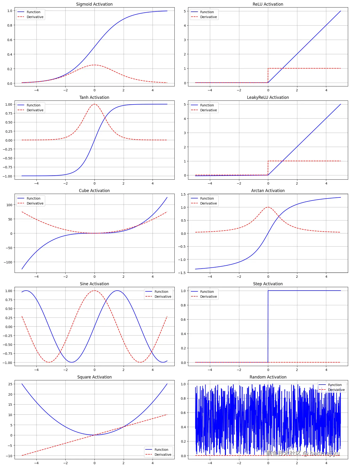
简介：

1. Sigmoid（标准激活函数）

数学形式： <math xmlns="http://www.w3.org/1998/Math/MathML"> f ( x ) = 1 1 + e − x f(x)=\dfrac{1}{1+e^{-x}} </math>f(x)=1+e−x1
特性：
- 输出范围在 <math xmlns="http://www.w3.org/1998/Math/MathML"> ( 0 , 1 ) (0,1) </math>(0,1) 之间，像"挤压"函数
- 将任意实数映射到 <math xmlns="http://www.w3.org/1998/Math/MathML"> 0 0 </math>0 到 <math xmlns="http://www.w3.org/1998/Math/MathML"> 1 1 </math>1 的概率区间
- 导数为 <math xmlns="http://www.w3.org/1998/Math/MathML"> f ′ ( x ) = f ( x ) ⋅ ( 1 − f ( x ) ) f'(x)=f(x)\cdot(1-f(x)) </math>f′(x)=f(x)⋅(1−f(x))
常见用途：
- 二分类问题的输出层（逻辑回归）
- 早期的神经网络隐藏层（现在较少使用）
缺点：
- 存在"梯度消失"问题：当 <math xmlns="http://www.w3.org/1998/Math/MathML"> ∣ x ∣ |x| </math>∣x∣较大时，梯度接近 <math xmlns="http://www.w3.org/1998/Math/MathML"> 0 0 </math>0
- 输出不是以 <math xmlns="http://www.w3.org/1998/Math/MathML"> 0 0 </math>0 为中心的，可能导致训练变慢
形象比喻：像一个"渐变开关"，从完全关闭(0)到完全打开(1)之间平滑过渡。

2. ReLU（标准激活函数）

数学形式： <math xmlns="http://www.w3.org/1998/Math/MathML"> f ( x ) = max ⁡ ( 0 , x ) f(x)=\max(0,x) </math>f(x)=max(0,x)
特性：
- 正数直接通过，负数变为 <math xmlns="http://www.w3.org/1998/Math/MathML"> 0 0 </math>0
- 计算非常简单高效
- 导数： <math xmlns="http://www.w3.org/1998/Math/MathML"> x > 0 x>0 </math>x>0 时为 <math xmlns="http://www.w3.org/1998/Math/MathML"> 1 1 </math>1， <math xmlns="http://www.w3.org/1998/Math/MathML"> x ≤ 0 x≤0 </math>x≤0时为 <math xmlns="http://www.w3.org/1998/Math/MathML"> 0 0 </math>0
常见用途：
- 现代深度神经网络的默认选择
- 几乎所有的卷积神经网络和全连接网络隐藏层
优点：
- 缓解了梯度消失问题（正区间梯度恒为 <math xmlns="http://www.w3.org/1998/Math/MathML"> 1 1 </math>1）
- 计算速度快（不需要指数运算）
- 稀疏激活（约 <math xmlns="http://www.w3.org/1998/Math/MathML"> 50 % 50\% </math>50%的神经元被激活）
缺点：
- "死亡ReLU"问题：负输入时梯度为 <math xmlns="http://www.w3.org/1998/Math/MathML"> 0 0 </math>0，神经元可能永久失活
- 输出不是以0为中心的

3. Tanh（标准激活函数）

数学形式： <math xmlns="http://www.w3.org/1998/Math/MathML"> f ( x ) = tanh ⁡ ( x ) = e x − e − x e x + e − x f(x)=\tanh(x)=\dfrac{e^x-e^{-x}}{e^x+e^{-x}} </math>f(x)=tanh(x)=ex+e−xex−e−x
特性：
- 输出范围在 <math xmlns="http://www.w3.org/1998/Math/MathML"> ( − 1 , 1 ) (-1,1) </math>(−1,1) 之间
- 以 <math xmlns="http://www.w3.org/1998/Math/MathML"> 0 0 </math>0 为中心，比Sigmoid更受欢迎
- 导数为 <math xmlns="http://www.w3.org/1998/Math/MathML"> f ′ ( x ) = 1 − tanh ⁡ 2 ( x ) f'(x)=1-\tanh^2(x) </math>f′(x)=1−tanh2(x)
常见用途：
- 循环神经网络（RNN）中常用
- 需要输出有正有负的场景
优点：
- 以 <math xmlns="http://www.w3.org/1998/Math/MathML"> 0 0 </math>0 为中心，优化效果通常比Sigmoid好
- 梯度比Sigmoid更强（最大梯度为 <math xmlns="http://www.w3.org/1998/Math/MathML"> 1 1 </math>1）
缺点：
- 仍然存在梯度消失问题（当 <math xmlns="http://www.w3.org/1998/Math/MathML"> ∣ x ∣ |x| </math>∣x∣较大时）

4. Leaky ReLU（标准激活函数变体）

数学形式： <math xmlns="http://www.w3.org/1998/Math/MathML"> f ( x ) = { x , x > 0 α x , x ⩽ 0 f(x)=\left\{\begin{matrix} x,x>0 & \\ \alpha x,x\leqslant 0 & \end{matrix}\right. </math>f(x)={x,x>0αx,x⩽0

通常 <math xmlns="http://www.w3.org/1998/Math/MathML"> α = 0.01 \alpha=0.01 </math>α=0.01

特性：
- 解决死亡ReLU问题的改进版
- 负区间有小的斜率α，而不是完全为0
- 导数： <math xmlns="http://www.w3.org/1998/Math/MathML"> x > 0 x>0 </math>x>0 时为 <math xmlns="http://www.w3.org/1998/Math/MathML"> 1 1 </math>1， <math xmlns="http://www.w3.org/1998/Math/MathML"> x ≤ 0 x≤0 </math>x≤0 时为 <math xmlns="http://www.w3.org/1998/Math/MathML"> α \alpha </math>α
常见用途：
- 当担心ReLU神经元死亡时
- 特别是对初始化敏感的网络
优点：
- 解决了死亡ReLU问题
- 保持了ReLU的大部分优点
变体：还有Parametric ReLU（PReLU， <math xmlns="http://www.w3.org/1998/Math/MathML"> α α </math>α可学习）、Randomized ReLU等

5. Cube（我瞎编的）

数学形式： <math xmlns="http://www.w3.org/1998/Math/MathML"> f ( x ) = x 3 f(x)=x^3 </math>f(x)=x3
特性：
- 简单的三次多项式
- 保持输入的符号（负输入得负输出，正输入得正输出）
- 导数为 <math xmlns="http://www.w3.org/1998/Math/MathML"> f ′ ( x ) = 3 x 2 f'(x)=3x^2 </math>f′(x)=3x2
潜在问题：
- 梯度爆炸风险：当 <math xmlns="http://www.w3.org/1998/Math/MathML"> ∣ x ∣ > 1 |x|>1 </math>∣x∣>1时，梯度快速增大
- 梯度消失风险：当 <math xmlns="http://www.w3.org/1998/Math/MathML"> ∣ x ∣ < 1 |x|<1 </math>∣x∣<1时，梯度很小
- 非线性太强，可能难以优化
研究意义：探索多项式激活函数的可能性，实际中很少使用

6. Arctan（还是我瞎编的）

数学形式： <math xmlns="http://www.w3.org/1998/Math/MathML"> f ( x ) = arctan ⁡ ( x ) f(x)=\arctan(x) </math>f(x)=arctan(x)
特性：
- 输出范围在 <math xmlns="http://www.w3.org/1998/Math/MathML"> ( − π 2 , π 2 ) (-\dfrac{\pi}{2},\dfrac{\pi}{2}) </math>(−2π,2π)之间
- 平滑的S形曲线，类似Sigmoid但范围更广
- 导数为 <math xmlns="http://www.w3.org/1998/Math/MathML"> f ′ ( x ) = 1 1 + x 2 f'(x)=\dfrac{1}{1+x^2} </math>f′(x)=1+x21
优点：
- 计算相对简单（比Sigmoid/Tanh少指数运算）
- 输出有界，防止激活值过大
缺点：
- 梯度消失严重：当 <math xmlns="http://www.w3.org/1998/Math/MathML"> ∣ x ∣ |x| </math>∣x∣较大时，梯度接近 <math xmlns="http://www.w3.org/1998/Math/MathML"> 0 0 </math>0
- 在实际神经网络中很少使用

7. Sine（又是我瞎编的）

数学形式： <math xmlns="http://www.w3.org/1998/Math/MathML"> f ( x ) = sin ⁡ ( x ) f(x)=\sin(x) </math>f(x)=sin(x)
特性：
- 周期为 <math xmlns="http://www.w3.org/1998/Math/MathML"> 2 π 2π </math>2π的振荡函数
- 输出范围在 <math xmlns="http://www.w3.org/1998/Math/MathML"> [ − 1 , 1 ] [-1,1] </math>[−1,1] 之间
- 导数为 <math xmlns="http://www.w3.org/1998/Math/MathML"> f ′ ( x ) = cos ⁡ ( x ) f'(x)=\cos(x) </math>f′(x)=cos(x)
独特性质：
- 周期性：不同的 <math xmlns="http://www.w3.org/1998/Math/MathML"> x x </math>x 可能得到相同的输出
- 无限多解：对于给定输出 <math xmlns="http://www.w3.org/1998/Math/MathML"> y y </math>y ，有无限多个 <math xmlns="http://www.w3.org/1998/Math/MathML"> x x </math>x 满足 <math xmlns="http://www.w3.org/1998/Math/MathML"> sin ⁡ ( x ) = y \sin(x)=y </math>sin(x)=y
潜在应用：
- 处理周期性数据（如信号处理）
- 理论研究中探索周期激活函数的特性
主要问题：
- 优化困难：梯度也在 <math xmlns="http://www.w3.org/1998/Math/MathML"> − 1 -1 </math>−1 到 <math xmlns="http://www.w3.org/1998/Math/MathML"> 1 1 </math>1 之间振荡
- 可能陷入局部振荡，难以收敛

8. Step（阶跃函数，基础但不实用的激活函数）

数学形式： <math xmlns="http://www.w3.org/1998/Math/MathML"> f ( x ) = { 1 , x > 0 0 , x ⩽ 0 f(x)=\left\{\begin{matrix} 1,x>0 & \\ 0,x\leqslant 0 & \end{matrix}\right. </math>f(x)={1,x>00,x⩽0
特性：
- 最简单的二值激活函数
- 也称为"单位阶跃函数"或"Heaviside阶跃函数"
- 导数在 <math xmlns="http://www.w3.org/1998/Math/MathML"> x ≠ 0 x≠0 </math>x=0时为 <math xmlns="http://www.w3.org/1998/Math/MathML"> 0 0 </math>0，在 <math xmlns="http://www.w3.org/1998/Math/MathML"> x = 0 x=0 </math>x=0 处未定义
历史意义：
- 最早的人工神经元（感知机）使用此函数
- Frank Rosenblatt的感知机(1958)使用此激活函数
致命缺点：
- 无法使用梯度下降：导数几乎处处为 <math xmlns="http://www.w3.org/1998/Math/MathML"> 0 0 </math>0
- 无法进行反向传播学习
现代应用：
- 仅用于理论教学或特定的离散优化问题
- 在神经网络的实际训练中从不使用

9. Square（双是我瞎编的）

数学形式： <math xmlns="http://www.w3.org/1998/Math/MathML"> f ( x ) = x 2 f(x)=x^2 </math>f(x)=x2
特性：
- 简单的二次函数
- 总是非负输出（失去符号信息）
- 导数为 <math xmlns="http://www.w3.org/1998/Math/MathML"> f ′ ( x ) = 2 x f'(x)=2x </math>f′(x)=2x
问题：
- 符号丢失：负输入和正输入都得到正输出
- 梯度爆炸：当 <math xmlns="http://www.w3.org/1998/Math/MathML"> ∣ x ∣ |x| </math>∣x∣较大时，梯度线性增长
- 非单调：不是单调函数，可能导致优化困难
潜在价值：
- 在某些特定的对称性检测任务中可能有用
- 理论研究中的对照实验

10. Random（叕是我瞎编的😂）

数学形式：每次前向传播时生成均匀分布的随机数 <math xmlns="http://www.w3.org/1998/Math/MathML"> U ( 0 , 1 ) U(0,1) </math>U(0,1)
特性：
- 完全忽略输入：输出与输入 <math xmlns="http://www.w3.org/1998/Math/MathML"> x x </math>x 无关
- 每次调用都产生新的随机数
- 导数为 <math xmlns="http://www.w3.org/1998/Math/MathML"> 0 0 </math>0（因为没有可学习的关系）
这是什么鬼😂：
- 这实际上不是一个有效的激活函数
- 它破坏了神经网络的基本前提：输出应该是输入的函数
为什么存在：
- 可能作为"反例"或"基线"测试
- 演示如果没有激活函数（或激活函数失效）会发生什么
- 在教学中展示为什么激活函数需要是输入的确定函数
结果预测：
- 网络完全无法学习任何模式
- 权重更新是随机的（因为梯度方向随机）
- 纯属娱乐或测试框架的极端情况🤣

训练结果：

python 复制代码

===Activation: Sigmoid===
Epoch 0, Loss: 0.25000092611954267, Weights: [0.00241735 0.00378633], Bias: -0.006269492222504486, predicted: [0.5        0.50095051 0.50060773 0.50155823]
Epoch 1000, Loss: 0.0944596668023508, Weights: [1.1533111  1.15352574], Bias: -1.955973219719276, predicted: [0.12402721 0.30956372 0.30951777 0.58669022]
Epoch 2000, Loss: 0.059342507126397645, Weights: [1.81421071 1.81425231], Bias: -2.8795553515206485, predicted: [0.0532118  0.2563415  0.25633355 0.67887591]
Epoch 3000, Loss: 0.04244503795960389, Weights: [2.26589322 2.26590371], Bias: -3.5355275860307978, predicted: [0.02833376 0.21935251 0.21935072 0.73028332]
Epoch 4000, Loss: 0.03251315255673547, Weights: [2.61066077 2.61066406], Bias: -4.041907016023551, predicted: [0.01726844 0.19292769 0.19292718 0.76481407]
Epoch 5000, Loss: 0.02606212211024169, Weights: [2.88798548 2.8879867 ], Bias: -4.451302760110763, predicted: [0.01153313 0.17318857 0.17318839 0.78993578]
Epoch 6000, Loss: 0.021587065559464505, Weights: [3.118719   3.11871952], Bias: -4.792900066901474, predicted: [0.00822282 0.15788119 0.15788112 0.80913951]
Epoch 7000, Loss: 0.018328942327454342, Weights: [3.31546126 3.3154615 ], Bias: -5.08471757342172, predicted: [0.00615421 0.14564588 0.14564585 0.82435132]
Epoch 8000, Loss: 0.015866402576175942, Weights: [3.48642116 3.48642128], Bias: -5.338627830705421, predicted: [0.00478063 0.13562315 0.13562314 0.83673494]
Epoch 9000, Loss: 0.013948780716040273, Weights: [3.63722897 3.63722904], Bias: -5.562829284210701, predicted: [0.00382403 0.12724606 0.12724605 0.84703797]
Epoch 10000, Loss: 0.012418682326926778, Weights: [3.77190017 3.77190021], Bias: -5.763195259016104, predicted: [0.00313182 0.12012651 0.12012651 0.85576351]
Predictions for Sigmoid: [0.00313122 0.12011992 0.12011992 0.85577157]

===Activation: ReLU===
Epoch 0, Loss: 0.25, Weights: [-0.01056155 -0.00261052], Bias: 0.0, predicted: [0. 0. 0. 0.]
Epoch 1000, Loss: 0.25, Weights: [-0.01056155 -0.00261052], Bias: 0.0, predicted: [0. 0. 0. 0.]
Epoch 2000, Loss: 0.25, Weights: [-0.01056155 -0.00261052], Bias: 0.0, predicted: [0. 0. 0. 0.]
Epoch 3000, Loss: 0.25, Weights: [-0.01056155 -0.00261052], Bias: 0.0, predicted: [0. 0. 0. 0.]
Epoch 4000, Loss: 0.25, Weights: [-0.01056155 -0.00261052], Bias: 0.0, predicted: [0. 0. 0. 0.]
Epoch 5000, Loss: 0.25, Weights: [-0.01056155 -0.00261052], Bias: 0.0, predicted: [0. 0. 0. 0.]
Epoch 6000, Loss: 0.25, Weights: [-0.01056155 -0.00261052], Bias: 0.0, predicted: [0. 0. 0. 0.]
Epoch 7000, Loss: 0.25, Weights: [-0.01056155 -0.00261052], Bias: 0.0, predicted: [0. 0. 0. 0.]
Epoch 8000, Loss: 0.25, Weights: [-0.01056155 -0.00261052], Bias: 0.0, predicted: [0. 0. 0. 0.]
Epoch 9000, Loss: 0.25, Weights: [-0.01056155 -0.00261052], Bias: 0.0, predicted: [0. 0. 0. 0.]
Epoch 10000, Loss: 0.25, Weights: [-0.01056155 -0.00261052], Bias: 0.0, predicted: [0. 0. 0. 0.]
Predictions for ReLU: [0. 0. 0. 0.]

===Activation: Tanh===
Epoch 0, Loss: 0.2517795840508127, Weights: [0.02746168 0.01927042], Bias: 0.02517628905913671, predicted: [ 0.         -0.00596666  0.00243455 -0.00353217]
Epoch 1000, Loss: 0.07822395248174475, Weights: [0.49070044 0.49070044], Bias: -0.24534865610195192, predicted: [-0.24054134  0.24054433  0.24054433  0.62675407]
Epoch 2000, Loss: 0.07822395247936782, Weights: [0.49070292 0.49070292], Bias: -0.24535145930358765, predicted: [-0.24054402  0.24054402  0.24054402  0.62675539]
Epoch 3000, Loss: 0.07822395247936781, Weights: [0.49070292 0.49070292], Bias: -0.24535145932872152, predicted: [-0.24054402  0.24054402  0.24054402  0.62675539]
Epoch 4000, Loss: 0.07822395247936781, Weights: [0.49070292 0.49070292], Bias: -0.24535145932872152, predicted: [-0.24054402  0.24054402  0.24054402  0.62675539]
Epoch 5000, Loss: 0.07822395247936781, Weights: [0.49070292 0.49070292], Bias: -0.24535145932872152, predicted: [-0.24054402  0.24054402  0.24054402  0.62675539]
Epoch 6000, Loss: 0.07822395247936781, Weights: [0.49070292 0.49070292], Bias: -0.24535145932872152, predicted: [-0.24054402  0.24054402  0.24054402  0.62675539]
Epoch 7000, Loss: 0.07822395247936781, Weights: [0.49070292 0.49070292], Bias: -0.24535145932872152, predicted: [-0.24054402  0.24054402  0.24054402  0.62675539]
Epoch 8000, Loss: 0.07822395247936781, Weights: [0.49070292 0.49070292], Bias: -0.24535145932872152, predicted: [-0.24054402  0.24054402  0.24054402  0.62675539]
Epoch 9000, Loss: 0.07822395247936781, Weights: [0.49070292 0.49070292], Bias: -0.24535145932872152, predicted: [-0.24054402  0.24054402  0.24054402  0.62675539]
Epoch 10000, Loss: 0.07822395247936781, Weights: [0.49070292 0.49070292], Bias: -0.24535145932872152, predicted: [-0.24054402  0.24054402  0.24054402  0.62675539]
Predictions for Tanh: [-0.24054402  0.24054402  0.24054402  0.62675539]

===Activation: LeakyReLU===
Epoch 0, Loss: 0.25007584551049644, Weights: [-0.01264564 -0.00202134], Bias: 0.00025007583547301384, predicted: [ 0.00000000e+00 -2.27138360e-05 -1.28957110e-04 -1.51670946e-04]
Epoch 1000, Loss: 5.2927938486298375e-05, Weights: [0.98709647 0.98709647], Bias: -0.9817348128367214, predicted: [-0.00981657  0.00538433  0.00538433  0.99242605]
Epoch 2000, Loss: 2.4997647353946023e-05, Weights: [0.99962766 0.99962766], Bias: -0.9994562789721012, predicted: [-9.99455228e-03  1.71685250e-04  1.71685250e-04  9.99798599e-01]
Epoch 3000, Loss: 2.4992503196942458e-05, Weights: [0.99979772 0.99979772], Bias: -0.9996967811565775, predicted: [-9.99696767e-03  1.00943273e-04  1.00943273e-04  9.99898653e-01]
Epoch 4000, Loss: 2.4992502249499728e-05, Weights: [0.99980003 0.99980003], Bias: -0.9997000450682826, predicted: [-9.99700045e-03  9.99832174e-05  9.99832174e-05  9.99900011e-01]
Epoch 5000, Loss: 2.4992502249325233e-05, Weights: [0.99980006 0.99980006], Bias: -0.9997000893635959, predicted: [-9.99700089e-03  9.99701883e-05  9.99701883e-05  9.99900030e-01]
Epoch 6000, Loss: 2.4992502249325202e-05, Weights: [0.99980006 0.99980006], Bias: -0.9997000899647376, predicted: [-9.99700090e-03  9.99700114e-05  9.99700114e-05  9.99900030e-01]
Epoch 7000, Loss: 2.4992502249325202e-05, Weights: [0.99980006 0.99980006], Bias: -0.999700089972893, predicted: [-9.9970009e-03  9.9970009e-05  9.9970009e-05  9.9990003e-01]
Epoch 8000, Loss: 2.4992502249325206e-05, Weights: [0.99980006 0.99980006], Bias: -0.9997000899729929, predicted: [-9.9970009e-03  9.9970009e-05  9.9970009e-05  9.9990003e-01]
Epoch 9000, Loss: 2.4992502249325206e-05, Weights: [0.99980006 0.99980006], Bias: -0.9997000899729929, predicted: [-9.9970009e-03  9.9970009e-05  9.9970009e-05  9.9990003e-01]
Epoch 10000, Loss: 2.4992502249325206e-05, Weights: [0.99980006 0.99980006], Bias: -0.9997000899729929, predicted: [-9.9970009e-03  9.9970009e-05  9.9970009e-05  9.9990003e-01]
Predictions for LeakyReLU: [-9.9970009e-03  9.9970009e-05  9.9970009e-05  9.9990003e-01]

===Activation: Cube===
Epoch 0, Loss: 0.25000004697016426, Weights: [ 0.00527862 -0.00982139], Bias: 1.5498741158811781e-06, predicted: [ 0.00000000e+00 -9.47816115e-07  1.46953117e-07 -9.39398641e-08]
Epoch 1000, Loss: 0.2500000056687841, Weights: [ 0.00604391 -0.0090561 ], Bias: 0.0007668393568271124, predicted: [ 4.50266807e-10 -5.69725811e-07  3.15819630e-07 -1.13373559e-08]
Epoch 2000, Loss: 0.2500000016608053, Weights: [ 0.00629518 -0.00880482], Bias: 0.0010181171310394612, predicted: [ 1.05482292e-09 -4.72189499e-07  3.91093332e-07 -3.32142272e-09]
Epoch 3000, Loss: 0.2500000006968277, Weights: [ 0.00642013 -0.00867987], Bias: 0.0011430682293705457, predicted: [ 1.49317190e-09 -4.28146870e-07  4.32597794e-07 -1.39347032e-09]
Epoch 4000, Loss: 0.2500000003556523, Weights: [ 0.00649488 -0.00860511], Bias: 0.0012178232978134473, predicted: [ 1.80588008e-09 -4.03158288e-07  4.58775626e-07 -7.11117981e-10]
Epoch 5000, Loss: 0.25000000020541285, Weights: [ 0.00654463 -0.00855536], Bias: 0.0012675713585682323, predicted: [ 2.03645428e-09 -3.87080896e-07  4.76767363e-07 -4.10637097e-10]
Epoch 6000, Loss: 0.2500000001291945, Weights: [ 0.00658012 -0.00851986], Bias: 0.0013030626458581261, predicted: [ 2.21240932e-09 -3.75876603e-07  4.89885665e-07 -2.58198395e-10]
Epoch 7000, Loss: 0.2500000000864845, Weights: [ 0.00660671 -0.00849327], Bias: 0.0013296577016542854, predicted: [ 2.35069760e-09 -3.67624230e-07  4.99871429e-07 -1.72776421e-10]
Epoch 8000, Loss: 0.25000000006071726, Weights: [ 0.00662738 -0.00847259], Bias: 0.0013503289098575298, predicted: [ 2.46207326e-09 -3.61294212e-07  5.07725684e-07 -1.21240350e-10]
Epoch 9000, Loss: 0.2500000000442594, Weights: [ 0.00664391 -0.00845606], Bias: 0.0013668571609993607, predicted: [ 2.55361382e-09 -3.56285511e-07  5.14064434e-07 -8.83230747e-11]
Epoch 10000, Loss: 0.2500000000332591, Weights: [ 0.00665743 -0.00844254], Bias: 0.0013803744991956, predicted: [ 2.63014193e-09 -3.52223822e-07  5.19287364e-07 -6.63213082e-11]
Predictions for Cube: [ 2.63021217e-09 -3.52220145e-07  5.19292127e-07 -6.63031904e-11]

===Activation: Arctan===
Epoch 0, Loss: 0.24126558320296862, Weights: [0.02519278 0.04123411], Bias: 0.024103693401520503, predicted: [0.         0.01711221 0.00066141 0.01777341]
Epoch 1000, Loss: 0.07678214225949234, Weights: [0.49819228 0.49819228], Bias: -0.2490943794364964, predicted: [-0.2441261   0.24412945  0.24412945  0.64176454]
Epoch 2000, Loss: 0.07678214225645766, Weights: [0.4981951 0.4981951], Bias: -0.24909754750487004, predicted: [-0.24412912  0.24412912  0.24412912  0.64176615]
Epoch 3000, Loss: 0.07678214225645766, Weights: [0.4981951 0.4981951], Bias: -0.2490975475368739, predicted: [-0.24412912  0.24412912  0.24412912  0.64176615]
Epoch 4000, Loss: 0.07678214225645766, Weights: [0.4981951 0.4981951], Bias: -0.2490975475368739, predicted: [-0.24412912  0.24412912  0.24412912  0.64176615]
Epoch 5000, Loss: 0.07678214225645766, Weights: [0.4981951 0.4981951], Bias: -0.2490975475368739, predicted: [-0.24412912  0.24412912  0.24412912  0.64176615]
Epoch 6000, Loss: 0.07678214225645766, Weights: [0.4981951 0.4981951], Bias: -0.2490975475368739, predicted: [-0.24412912  0.24412912  0.24412912  0.64176615]
Epoch 7000, Loss: 0.07678214225645766, Weights: [0.4981951 0.4981951], Bias: -0.2490975475368739, predicted: [-0.24412912  0.24412912  0.24412912  0.64176615]
Epoch 8000, Loss: 0.07678214225645766, Weights: [0.4981951 0.4981951], Bias: -0.2490975475368739, predicted: [-0.24412912  0.24412912  0.24412912  0.64176615]
Epoch 9000, Loss: 0.07678214225645766, Weights: [0.4981951 0.4981951], Bias: -0.2490975475368739, predicted: [-0.24412912  0.24412912  0.24412912  0.64176615]
Epoch 10000, Loss: 0.07678214225645766, Weights: [0.4981951 0.4981951], Bias: -0.2490975475368739, predicted: [-0.24412912  0.24412912  0.24412912  0.64176615]
Predictions for Arctan: [-0.24412912  0.24412912  0.24412912  0.64176615]

===Activation: Sine===
Epoch 0, Loss: 0.25048530595694735, Weights: [0.02571101 0.02339311], Bias: 0.02504841297015858, predicted: [ 0.         -0.00167292  0.00070442 -0.0009685 ]
Epoch 1000, Loss: 0.0712340695646528, Weights: [0.49569736 0.49569736], Bias: -0.2478483300106123, predicted: [-0.2453186   0.24531928  0.24531928  0.67690255]
Epoch 2000, Loss: 0.07123406956452127, Weights: [0.4956979 0.4956979], Bias: -0.24784894931868487, predicted: [-0.24531921  0.24531921  0.24531921  0.6769029 ]
Epoch 3000, Loss: 0.07123406956452126, Weights: [0.4956979 0.4956979], Bias: -0.2478489493197496, predicted: [-0.24531921  0.24531921  0.24531921  0.6769029 ]
Epoch 4000, Loss: 0.07123406956452126, Weights: [0.4956979 0.4956979], Bias: -0.2478489493197496, predicted: [-0.24531921  0.24531921  0.24531921  0.6769029 ]
Epoch 5000, Loss: 0.07123406956452126, Weights: [0.4956979 0.4956979], Bias: -0.2478489493197496, predicted: [-0.24531921  0.24531921  0.24531921  0.6769029 ]
Epoch 6000, Loss: 0.07123406956452126, Weights: [0.4956979 0.4956979], Bias: -0.2478489493197496, predicted: [-0.24531921  0.24531921  0.24531921  0.6769029 ]
Epoch 7000, Loss: 0.07123406956452126, Weights: [0.4956979 0.4956979], Bias: -0.2478489493197496, predicted: [-0.24531921  0.24531921  0.24531921  0.6769029 ]
Epoch 8000, Loss: 0.07123406956452126, Weights: [0.4956979 0.4956979], Bias: -0.2478489493197496, predicted: [-0.24531921  0.24531921  0.24531921  0.6769029 ]
Epoch 9000, Loss: 0.07123406956452126, Weights: [0.4956979 0.4956979], Bias: -0.2478489493197496, predicted: [-0.24531921  0.24531921  0.24531921  0.6769029 ]
Epoch 10000, Loss: 0.07123406956452126, Weights: [0.4956979 0.4956979], Bias: -0.2478489493197496, predicted: [-0.24531921  0.24531921  0.24531921  0.6769029 ]
Predictions for Sine: [-0.24531921  0.24531921  0.24531921  0.6769029 ]

===Activation: Step===
Epoch 0, Loss: 0.75, Weights: [0.00442023 0.00111435], Bias: 0.0, predicted: [1 1 1 1]
Epoch 1000, Loss: 0.75, Weights: [0.00442023 0.00111435], Bias: 0.0, predicted: [1 1 1 1]
Epoch 2000, Loss: 0.75, Weights: [0.00442023 0.00111435], Bias: 0.0, predicted: [1 1 1 1]
Epoch 3000, Loss: 0.75, Weights: [0.00442023 0.00111435], Bias: 0.0, predicted: [1 1 1 1]
Epoch 4000, Loss: 0.75, Weights: [0.00442023 0.00111435], Bias: 0.0, predicted: [1 1 1 1]
Epoch 5000, Loss: 0.75, Weights: [0.00442023 0.00111435], Bias: 0.0, predicted: [1 1 1 1]
Epoch 6000, Loss: 0.75, Weights: [0.00442023 0.00111435], Bias: 0.0, predicted: [1 1 1 1]
Epoch 7000, Loss: 0.75, Weights: [0.00442023 0.00111435], Bias: 0.0, predicted: [1 1 1 1]
Epoch 8000, Loss: 0.75, Weights: [0.00442023 0.00111435], Bias: 0.0, predicted: [1 1 1 1]
Epoch 9000, Loss: 0.75, Weights: [0.00442023 0.00111435], Bias: 0.0, predicted: [1 1 1 1]
Epoch 10000, Loss: 0.75, Weights: [0.00442023 0.00111435], Bias: 0.0, predicted: [1 1 1 1]
Predictions for Step: [1 1 1 1]

===Activation: Square===
Epoch 0, Loss: 0.249901981437154, Weights: [-0.01365194 -0.00175044], Bias: -0.0006998797660097009, predicted: [0.00000000e+00 1.10345213e-06 1.67755896e-04 1.96070419e-04]
Epoch 1000, Loss: 0.008928571428910015, Weights: [-0.65465299 -0.65465299], Bias: 0.32732566867964547, predicted: [0.10714208 0.10714318 0.10714318 0.96428534]
Epoch 2000, Loss: 0.008928571428571428, Weights: [-0.65465367 -0.65465367], Bias: 0.32732683535342944, predicted: [0.10714286 0.10714286 0.10714286 0.96428571]
Epoch 3000, Loss: 0.008928571428571428, Weights: [-0.65465367 -0.65465367], Bias: 0.3273268353539852, predicted: [0.10714286 0.10714286 0.10714286 0.96428571]
Epoch 4000, Loss: 0.008928571428571428, Weights: [-0.65465367 -0.65465367], Bias: 0.3273268353539852, predicted: [0.10714286 0.10714286 0.10714286 0.96428571]
Epoch 5000, Loss: 0.008928571428571428, Weights: [-0.65465367 -0.65465367], Bias: 0.3273268353539852, predicted: [0.10714286 0.10714286 0.10714286 0.96428571]
Epoch 6000, Loss: 0.008928571428571428, Weights: [-0.65465367 -0.65465367], Bias: 0.3273268353539852, predicted: [0.10714286 0.10714286 0.10714286 0.96428571]
Epoch 7000, Loss: 0.008928571428571428, Weights: [-0.65465367 -0.65465367], Bias: 0.3273268353539852, predicted: [0.10714286 0.10714286 0.10714286 0.96428571]
Epoch 8000, Loss: 0.008928571428571428, Weights: [-0.65465367 -0.65465367], Bias: 0.3273268353539852, predicted: [0.10714286 0.10714286 0.10714286 0.96428571]
Epoch 9000, Loss: 0.008928571428571428, Weights: [-0.65465367 -0.65465367], Bias: 0.3273268353539852, predicted: [0.10714286 0.10714286 0.10714286 0.96428571]
Epoch 10000, Loss: 0.008928571428571428, Weights: [-0.65465367 -0.65465367], Bias: 0.3273268353539852, predicted: [0.10714286 0.10714286 0.10714286 0.96428571]
Predictions for Square: [0.10714286 0.10714286 0.10714286 0.96428571]

===Activation: Random===
Epoch 0, Loss: 0.2949918655654963, Weights: [-0.01852296  0.01947434], Bias: 0.0, predicted: [0.63615563 0.25606144 0.5159263  0.33402248]
Epoch 1000, Loss: 0.27114951738689796, Weights: [-0.01852296  0.01947434], Bias: 0.0, predicted: [0.45244767 0.51022229 0.33801333 0.28914884]
Epoch 2000, Loss: 0.36495140334118076, Weights: [-0.01852296  0.01947434], Bias: 0.0, predicted: [0.78509413 0.23504109 0.87499173 0.84974029]
Epoch 3000, Loss: 0.387758559664891, Weights: [-0.01852296  0.01947434], Bias: 0.0, predicted: [0.01715636 0.97493812 0.59400479 0.50261295]
Epoch 4000, Loss: 0.3872913395162145, Weights: [-0.01852296  0.01947434], Bias: 0.0, predicted: [0.5666904  0.21683046 0.96591912 0.50199181]
Epoch 5000, Loss: 0.25004964539235475, Weights: [-0.01852296  0.01947434], Bias: 0.0, predicted: [0.85291767 0.26381048 0.37232479 0.74601514]
Epoch 6000, Loss: 0.2022779138555904, Weights: [-0.01852296  0.01947434], Bias: 0.0, predicted: [0.40811267 0.52478263 0.36221412 0.51424304]
Epoch 7000, Loss: 0.3191685815801508, Weights: [-0.01852296  0.01947434], Bias: 0.0, predicted: [0.74127179 0.1535808  0.3429831  0.23451584]
Epoch 8000, Loss: 0.5615845931155097, Weights: [-0.01852296  0.01947434], Bias: 0.0, predicted: [0.78435424 0.74548253 0.99287256 0.70068967]
Epoch 9000, Loss: 0.039691524453809975, Weights: [-0.01852296  0.01947434], Bias: 0.0, predicted: [0.07853389 0.23117278 0.24828647 0.80632113]
Epoch 10000, Loss: 0.3710152109550447, Weights: [-0.01852296  0.01947434], Bias: 0.0, predicted: [0.6720607  0.17746654 0.43058438 0.09695074]
Predictions for Random: [0.87954606 0.15693083 0.41057489 0.61516742]

训练轮数 <math xmlns="http://www.w3.org/1998/Math/MathML"> 10000 10000 </math>10000轮，学习率 <math xmlns="http://www.w3.org/1998/Math/MathML"> 0.1 0.1 </math>0.1，训练用时 <math xmlns="http://www.w3.org/1998/Math/MathML"> 0.8 0.8 </math>0.8秒

结果非常amazing啊！ 好几个我瞎编的函数训练效果都不错😹。另外LeakyReLU的训练效果极好，其一万轮训练后的损失来到了约 <math xmlns="http://www.w3.org/1998/Math/MathML"> 2.5 e − 05 2.5e-05 </math>2.5e−05，而Sigmoid需要 <math xmlns="http://www.w3.org/1998/Math/MathML"> 681 681 </math>681万轮训练才能达到同样效果（测试Sigmoid 训练用时 <math xmlns="http://www.w3.org/1998/Math/MathML"> 50.0 s 50.0s </math>50.0s ）

可视化：

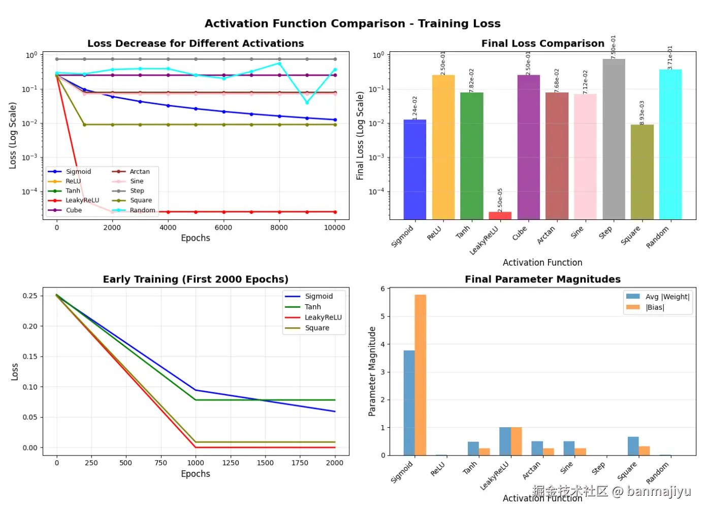
📊 整体评分表

激活函数	收敛性	正确性	稳定性	学习效率	综合评分	备注
Sigmoid	3/5	4/5	5/5	3/5	15/20	稳定收敛，正确分类但不够精确
ReLU	1/5	1/5	5/5	1/5	8/20	神经元死亡，完全无法学习
Tanh	3/5	2/5	5/5	3/5	13/20	稳定收敛但分类错误
LeakyReLU	5/5	5/5	5/5	5/5	20/20	最佳表现：快速收敛，完美分类
Cube	1/5	1/5	5/5	1/5	8/20	几乎不学习，梯度太小
Arctan	3/5	2/5	5/5	3/5	13/20	稳定收敛但分类错误
Sine	3/5	2/5	5/5	3/5	13/20	稳定收敛但分类错误
Step	1/5	1/5	5/5	1/5	8/20	梯度为0，完全无法学习
Square	4/5	4/5	5/5	4/5	17/20	良好收敛，正确分类但不够精确
Random	1/5	1/5	1/5	1/5	4/20	完全随机，无学习能力

🔍 详细分析

Sigmoid
- 收敛性：✅ 损失从 <math xmlns="http://www.w3.org/1998/Math/MathML"> 0.25 0.25 </math>0.25稳步降至 <math xmlns="http://www.w3.org/1998/Math/MathML"> 0.012 0.012 </math>0.012，下降趋势良好但速度较慢。
- 参数演变：权重从 <math xmlns="http://www.w3.org/1998/Math/MathML"> ≈ 0 ≈0 </math>≈0增至 <math xmlns="http://www.w3.org/1998/Math/MathML"> ≈ 3.77 ≈3.77 </math>≈3.77，偏置从 <math xmlns="http://www.w3.org/1998/Math/MathML"> ≈ 0 ≈0 </math>≈0降至 <math xmlns="http://www.w3.org/1998/Math/MathML"> ≈ − 5.76 ≈-5.76 </math>≈−5.76，持续增长。
- 正确性：预测值 <math xmlns="http://www.w3.org/1998/Math/MathML"> [ 0.0031 , 0.1201 , 0.1201 , 0.8558 ] [0.0031, 0.1201, 0.1201, 0.8558] </math>[0.0031,0.1201,0.1201,0.8558]，以 <math xmlns="http://www.w3.org/1998/Math/MathML"> 0.5 0.5 </math>0.5为阈值分类完全正确。
- 特点：典型的S形激活函数，输出范围 <math xmlns="http://www.w3.org/1998/Math/MathML"> ( 0 , 1 ) (0,1) </math>(0,1)天然适合概率解释。学习率 <math xmlns="http://www.w3.org/1998/Math/MathML"> 0.1 0.1 </math>0.1较合适，但 <math xmlns="http://www.w3.org/1998/Math/MathML"> 10000 10000 </math>10000轮仍未完全收敛，可增加轮数。
ReLU
- 收敛性：❌ 完全失败！损失恒为 <math xmlns="http://www.w3.org/1998/Math/MathML"> 0.25 0.25 </math>0.25，从未下降。
- 参数演变：参数几乎不变，训练一开始就停滞。
- 问题根源：神经元死亡。ReLU在负输入时梯度为 <math xmlns="http://www.w3.org/1998/Math/MathML"> 0 0 </math>0，而AND运算需要负偏置使 <math xmlns="http://www.w3.org/1998/Math/MathML"> ( 0 , 0 ) 、 ( 0 , 1 ) 、 ( 1 , 0 ) (0,0)、(0,1)、(1,0) </math>(0,0)、(0,1)、(1,0)输出为负。一旦线性输出为负，ReLU输出 <math xmlns="http://www.w3.org/1998/Math/MathML"> 0 0 </math>0且梯度为 <math xmlns="http://www.w3.org/1998/Math/MathML"> 0 0 </math>0，参数无法更新。
- 教训：ReLU不适合用于单层感知机的输出层，特别当需要负输出时。
Tanh
- 收敛性：✅ 损失从 <math xmlns="http://www.w3.org/1998/Math/MathML"> 0.252 0.252 </math>0.252降至 <math xmlns="http://www.w3.org/1998/Math/MathML"> 0.078 0.078 </math>0.078并稳定。
- 参数演变：权重稳定在 <math xmlns="http://www.w3.org/1998/Math/MathML"> ≈ 0.49 ≈0.49 </math>≈0.49，偏置 <math xmlns="http://www.w3.org/1998/Math/MathML"> ≈ − 0.245 ≈-0.245 </math>≈−0.245，对称但值较小。
- 正确性：预测值 <math xmlns="http://www.w3.org/1998/Math/MathML"> [ − 0.2405 , 0.2405 , 0.2405 , 0.6268 ] [-0.2405, 0.2405, 0.2405, 0.6268] </math>[−0.2405,0.2405,0.2405,0.6268]，以0为阈值时分类错误（ <math xmlns="http://www.w3.org/1998/Math/MathML"> ( 0 , 1 ) (0,1) </math>(0,1)和 <math xmlns="http://www.w3.org/1998/Math/MathML"> ( 1 , 0 ) (1,0) </math>(1,0)被预测为正）。
- 分析：Tanh输出范围 <math xmlns="http://www.w3.org/1998/Math/MathML"> ( − 1 , 1 ) (-1,1) </math>(−1,1)，但标签为 <math xmlns="http://www.w3.org/1998/Math/MathML"> { 0 , 1 } \{0,1\} </math>{0,1}，模型尝试将负例映射到负值，但未成功分离 <math xmlns="http://www.w3.org/1998/Math/MathML"> ( 0 , 1 ) (0,1) </math>(0,1)和 <math xmlns="http://www.w3.org/1998/Math/MathML"> ( 1 , 0 ) (1,0) </math>(1,0)。需要调整标签为 <math xmlns="http://www.w3.org/1998/Math/MathML"> { − 1 , 1 } \{-1,1\} </math>{−1,1}或修改决策阈值。
LeakyReLU ⭐ 最佳表现
- 收敛性：✅✅ 极佳！损失从 <math xmlns="http://www.w3.org/1998/Math/MathML"> 0.2501 0.2501 </math>0.2501迅速降至 <math xmlns="http://www.w3.org/1998/Math/MathML"> 2.5 e − 5 2.5e-5 </math>2.5e−5。
- 参数演变：权重快速收敛到 <math xmlns="http://www.w3.org/1998/Math/MathML"> ≈ 1.0 ≈1.0 </math>≈1.0，偏置到 <math xmlns="http://www.w3.org/1998/Math/MathML"> ≈ − 1.0 ≈-1.0 </math>≈−1.0，完美匹配AND的线性边界 <math xmlns="http://www.w3.org/1998/Math/MathML"> x 1 + x 2 − 1.5 x_1+x_2-1.5 </math>x1+x2−1.5。
- 正确性：预测值 <math xmlns="http://www.w3.org/1998/Math/MathML"> [ − 0.009997 , 0.0001 , 0.0001 , 0.9999 ] [-0.009997, 0.0001, 0.0001, 0.9999] </math>[−0.009997,0.0001,0.0001,0.9999]，几乎完美匹配 <math xmlns="http://www.w3.org/1998/Math/MathML"> [ 0 , 0 , 0 , 1 ] [0,0,0,1] </math>[0,0,0,1]。
- 优势：LeakyReLU（ <math xmlns="http://www.w3.org/1998/Math/MathML"> α = 0.01 α=0.01 </math>α=0.01）允许负梯度流动，避免了ReLU的死亡问题，且保持了ReLU的快速收敛特性。
Cube
- 收敛性：❌ 几乎不学习，损失从 <math xmlns="http://www.w3.org/1998/Math/MathML"> 0.25000005 0.25000005 </math>0.25000005降至 <math xmlns="http://www.w3.org/1998/Math/MathML"> 0.25000003 0.25000003 </math>0.25000003，变化微乎其微。
- 参数演变：参数变化极小，权重 <math xmlns="http://www.w3.org/1998/Math/MathML"> ≈ 0.0066 ≈0.0066 </math>≈0.0066，偏置 <math xmlns="http://www.w3.org/1998/Math/MathML"> ≈ 0.0014 ≈0.0014 </math>≈0.0014。
- 问题：立方函数的梯度为 <math xmlns="http://www.w3.org/1998/Math/MathML"> 3 x 2 3x^2 </math>3x2，当x接近0时梯度极小，导致更新极其缓慢。这是梯度消失的典型案例。
- 教训：单调但导数变化剧烈的激活函数可能导致优化困难。
Arctan
- 收敛性：✅ 类似Tanh，损失从 <math xmlns="http://www.w3.org/1998/Math/MathML"> 0.241 0.241 </math>0.241降至 <math xmlns="http://www.w3.org/1998/Math/MathML"> 0.077 0.077 </math>0.077并稳定。
- 参数演变：权重 <math xmlns="http://www.w3.org/1998/Math/MathML"> ≈ 0.498 ≈0.498 </math>≈0.498，偏置 <math xmlns="http://www.w3.org/1998/Math/MathML"> ≈ − 0.249 ≈-0.249 </math>≈−0.249，与Tanh非常相似。
- 正确性：预测值 <math xmlns="http://www.w3.org/1998/Math/MathML"> [ − 0.2441 , 0.2441 , 0.2441 , 0.6418 ] [-0.2441, 0.2441, 0.2441, 0.6418] </math>[−0.2441,0.2441,0.2441,0.6418]，同样分类错误。
- 分析：Arctan也是S形函数，输出范围 <math xmlns="http://www.w3.org/1998/Math/MathML"> ( − π 2 , π 2 ) (-\dfrac{\pi}{2}, \dfrac{\pi}{2}) </math>(−2π,2π)，与Tanh面临相同问题：输出范围不匹配二进制标签。
Sine
- 收敛性：✅ 损失从 <math xmlns="http://www.w3.org/1998/Math/MathML"> 0.2505 0.2505 </math>0.2505降至 <math xmlns="http://www.w3.org/1998/Math/MathML"> 0.0712 0.0712 </math>0.0712并稳定。
- 参数演变：权重 <math xmlns="http://www.w3.org/1998/Math/MathML"> ≈ 0.4957 ≈0.4957 </math>≈0.4957，偏置 <math xmlns="http://www.w3.org/1998/Math/MathML"> ≈ − 0.2478 ≈-0.2478 </math>≈−0.2478，与Tanh/Arctan同一量级。
- 正确性：预测值 <math xmlns="http://www.w3.org/1998/Math/MathML"> [ − 0.2453 , 0.2453 , 0.2453 , 0.6769 ] [-0.2453, 0.2453, 0.2453, 0.6769] </math>[−0.2453,0.2453,0.2453,0.6769]，分类错误。
- 特点：正弦函数的周期性没有被利用，反而收敛到一个类似Tanh的平衡点。对于线性可分问题，周期性激活函数没有优势。
Step
- 收敛性：❌ 完全失败，损失恒为 <math xmlns="http://www.w3.org/1998/Math/MathML"> 0.75 0.75 </math>0.75（最差可能值）。
- 参数演变：参数几乎不变，梯度处处为 <math xmlns="http://www.w3.org/1998/Math/MathML"> 0 0 </math>0。
- 问题：阶跃函数的导数（除 <math xmlns="http://www.w3.org/1998/Math/MathML"> x = 0 x=0 </math>x=0外）为 <math xmlns="http://www.w3.org/1998/Math/MathML"> 0 0 </math>0，梯度下降完全失效。这是感知机原始算法使用的激活函数，但无法用梯度下降训练。
- 历史意义：1958年Rosenblatt的感知机使用此函数，但需要特殊学习规则。
Square
- 收敛性：✅ 损失从 <math xmlns="http://www.w3.org/1998/Math/MathML"> 0.250 0.250 </math>0.250 降至 <math xmlns="http://www.w3.org/1998/Math/MathML"> 0.00893 0.00893 </math>0.00893，收敛良好。
- 参数演变：权重收敛到 <math xmlns="http://www.w3.org/1998/Math/MathML"> ≈ − 0.6547 ≈-0.6547 </math>≈−0.6547，偏置 <math xmlns="http://www.w3.org/1998/Math/MathML"> ≈ 0.3273 ≈0.3273 </math>≈0.3273（注意权重为负）。
- 正确性：预测值 <math xmlns="http://www.w3.org/1998/Math/MathML"> [ 0.1071 , 0.1071 , 0.1071 , 0.9643 ] [0.1071, 0.1071, 0.1071, 0.9643] </math>[0.1071,0.1071,0.1071,0.9643]，以0.5为阈值分类正确。
- 特点：平方函数总是输出非负值，但模型找到了一个解：使 <math xmlns="http://www.w3.org/1998/Math/MathML"> ( 0 , 0 ) 、 ( 0 , 1 ) 、 ( 1 , 0 ) (0,0)、(0,1)、(1,0) </math>(0,0)、(0,1)、(1,0)输出较小正值， <math xmlns="http://www.w3.org/1998/Math/MathML"> ( 1 , 1 ) (1,1) </math>(1,1)输出接近 <math xmlns="http://www.w3.org/1998/Math/MathML"> 1 1 </math>1。虽然数学上可行，但不够直观。
Random🤣
- 收敛性：❌ 完全随机，损失在 <math xmlns="http://www.w3.org/1998/Math/MathML"> 0.04 0.04 </math>0.04到 <math xmlns="http://www.w3.org/1998/Math/MathML"> 0.56 0.56 </math>0.56之间随机波动。
- 参数演变：参数不变（梯度为 <math xmlns="http://www.w3.org/1998/Math/MathML"> 0 0 </math>0），但输出每次随机。
- 问题：这不是真正的激活函数，输出与输入无关，完全没有学习能力。仅作为反例存在。

📈 警示

输出范围的重要性
- 匹配标签范围：Sigmoid <math xmlns="http://www.w3.org/1998/Math/MathML"> ( 0 , 1 ) (0,1) </math>(0,1)、LeakyReLU(允许负值)表现最佳，因为输出范围与二进制标签 <math xmlns="http://www.w3.org/1998/Math/MathML"> { 0 , 1 } \{0,1\} </math>{0,1}兼容或能跨越0点。
- 范围不匹配问题：Tanh、Arctan、Sine输出包含负值，但模型未能将负例映射到负值，因为MSE损失对称惩罚正负误差。
梯度特性决定学习能力
- 梯度消失：Cube在 <math xmlns="http://www.w3.org/1998/Math/MathML"> 0 0 </math>0 附近梯度极小，导致学习停滞。
- 梯度截断：ReLU在负区间梯度为 <math xmlns="http://www.w3.org/1998/Math/MathML"> 0 0 </math>0，导致神经元死亡。
- 梯度保持：LeakyReLU、Sigmoid在所有区域都有非零梯度，学习顺利。
决策边界可视化
- 成功的激活函数学习到的决策函数：
  - LeakyReLU： <math xmlns="http://www.w3.org/1998/Math/MathML"> f ( x ) = l e a k y _ r e l u ( x 1 + x 2 − 1 ) f(x) = \mathrm{leaky\_relu}(x_1 + x_2 - 1) </math>f(x)=leaky_relu(x1+x2−1)，阈值清晰
  - Sigmoid： <math xmlns="http://www.w3.org/1998/Math/MathML"> f ( x ) = σ ( w 1 x 1 + w 2 x 2 + b ) f(x) = \sigma(w_1x_1 + w_2x_2 + b) </math>f(x)=σ(w1x1+w2x2+b)，平滑过渡
  - Square： <math xmlns="http://www.w3.org/1998/Math/MathML"> f ( x ) = ( w 1 x 1 + w 2 x 2 + b ) 2 f(x) = (w_1x_1 + w_2x_2 + b)^2 </math>f(x)=(w1x1+w2x2+b)2，抛物线决策
学习率敏感性
- 所有实验中学习率固定为 <math xmlns="http://www.w3.org/1998/Math/MathML"> 0.1 0.1 </math>0.1
- Cube需要更小的学习率（梯度变化大）
- ReLU可能需要更大的初始权重避免死亡

🎯 实用建议

对于简单二分类：LeakyReLU或Sigmoid是最佳选择。
避免使用：Step（无法梯度下降）、Random（无意义）、Cube（梯度问题）。
输出层选择：二分类输出层应用Sigmoid，配合交叉熵损失而非MSE。
初始化重要性：ReLU的失败部分源于不良初始化，可尝试He初始化。
标签编码：使用Tanh类激活函数时，考虑将标签改为 <math xmlns="http://www.w3.org/1998/Math/MathML"> { − 1 , 1 } \{-1,1\} </math>{−1,1}。

这个实验展示了激活函数对神经网络学习能力的决定性影响。LeakyReLU在本任务中表现完美，而ReLU则因神经元死亡完全失败------这正是深度学习实践中ReLU需要谨慎使用的原因。

🤣谁说`Random`不行？🤣

激活函数是不会写代码的猴子才需要的，Random()才是永远的神！

python 复制代码

import numpy as np

class MonkeyPerceptron:
    def init(self):
        self.weights = None
        self.bias = None
        self.Loss = None
    
    def sigmoid(self, z):
        return 1 / (1 + np.exp(-z))

    def fit(self, X, y):
        num_samples, num_features = X.shape
        self.weights = np.zeros(num_features)
        self.bias = 0
        _ = 0
        while True:
            rand_weights = np.random.rand(num_features) * 10 # 随机权重
            rand_bias = - np.random.rand() * 50  # 随机偏置
            linear_model = np.dot(X, rand_weights) + rand_bias
            y_predicted = self.sigmoid(linear_model)    # 预测概率
            _ += 1
            loss = -np.mean(y * np.log(y_predicted + 1e-15) + (1 - y) * np.log(1 - y_predicted + 1e-15)) # 计算损失
            if self.Loss is None or loss < self.Loss:  # 更新权重和偏置
                self.Loss = loss
                self.weights = rand_weights
                self.bias = randbias
            
            print(f"===Epoch {}=== \nLoss: {loss:.6f}, Weight: {rand_weights}, Bias: {randbias}\nBestLoss: {self.Loss:.6f}, BestWeights: {self.weights}, BestBias: {self.bias}")

            if self.Loss is not None and self.Loss < 0.01:  # 如果损失足够小，停止训练
                print(f"最终：Epoch {}, Loss: {self.Loss:.6f}, Weights: {self.weights}, Bias: {self.bias}")
                break
            
    def predict(self, X):
        linear_model = np.dot(X, self.weights) + self.bias
        y_predicted = self.sigmoid(linear_model)
        y_predicted_cls = [i for i in y_predicted]
        return np.array(y_predicted_cls)
    
if name == "main":
    X = np.array([[0, 0],
                  [0, 1],
                  [1, 0],
                  [1, 1]])
    y = np.array([0, 0, 0, 1])  # labels

    perceptron = MonkeyPerceptron()
    perceptron.fit(X, y)
    res = perceptron.predict(X)
    print("Predictions:", res)

训练结果（训练用时 <math xmlns="http://www.w3.org/1998/Math/MathML"> 0.0 s 0.0s </math>0.0s）（别问我刷了多久🤣）：

python 复制代码

===Epoch 1=== 
Loss: 1.972791, Weight: [5.30602216 5.40416736], Bias: -1.5292279253220298
BestLoss: 1.972791, BestWeights: [5.30602216 5.40416736], BestBias: -1.5292279253220298
===Epoch 2=== 
Loss: 0.287885, Weight: [3.10076394 2.30376275], Bias: -6.063241275953091
BestLoss: 0.287885, BestWeights: [3.10076394 2.30376275], BestBias: -6.063241275953091
===Epoch 3=== 
Loss: 1.992203, Weight: [0.74941079 6.26557104], Bias: -14.983283585555174
BestLoss: 0.287885, BestWeights: [3.10076394 2.30376275], BestBias: -6.063241275953091
===Epoch 4=== 
Loss: 0.241579, Weight: [9.79877349 2.36787043], Bias: -12.55242733698611
BestLoss: 0.241579, BestWeights: [9.79877349 2.36787043], BestBias: -12.55242733698611
===Epoch 5=== 
Loss: 4.968945, Weight: [3.57131294 2.20885872], Bias: -25.65595066981524
BestLoss: 0.241579, BestWeights: [9.79877349 2.36787043], BestBias: -12.55242733698611
===Epoch 6=== 
Loss: 6.923904, Weight: [7.98137279 6.85191969], Bias: -42.529975532939034
BestLoss: 0.241579, BestWeights: [9.79877349 2.36787043], BestBias: -12.55242733698611
===Epoch 7=== 
Loss: 1.595178, Weight: [0.18703687 6.04751624], Bias: -0.6114760434528632
BestLoss: 0.241579, BestWeights: [9.79877349 2.36787043], BestBias: -12.55242733698611
===Epoch 8=== 
Loss: 1.949835, Weight: [7.42283631 4.89233456], Bias: -2.344499180233811
BestLoss: 0.241579, BestWeights: [9.79877349 2.36787043], BestBias: -12.55242733698611
===Epoch 9=== 
Loss: 4.815745, Weight: [1.33092208 7.4939571 ], Bias: -28.087861342745196
BestLoss: 0.241579, BestWeights: [9.79877349 2.36787043], BestBias: -12.55242733698611
===Epoch 10=== 
Loss: 8.634688, Weight: [0.03286126 3.13750956], Bias: -48.27619183591643
BestLoss: 0.241579, BestWeights: [9.79877349 2.36787043], BestBias: -12.55242733698611
===Epoch 11=== 
Loss: 8.628221, Weight: [0.08143696 7.54346519], Bias: -45.804449939873436
BestLoss: 0.241579, BestWeights: [9.79877349 2.36787043], BestBias: -12.55242733698611
===Epoch 12=== 
Loss: 0.543617, Weight: [2.68455094 3.80666757], Bias: -8.53157179318768
BestLoss: 0.241579, BestWeights: [9.79877349 2.36787043], BestBias: -12.55242733698611
===Epoch 13=== 
Loss: 0.807674, Weight: [8.3456054  3.90103381], Bias: -5.376559159273797
BestLoss: 0.241579, BestWeights: [9.79877349 2.36787043], BestBias: -12.55242733698611
===Epoch 14=== 
Loss: 1.459065, Weight: [1.39063704 4.99957087], Bias: -12.222789575320242
BestLoss: 0.241579, BestWeights: [9.79877349 2.36787043], BestBias: -12.55242733698611
===Epoch 15=== 
Loss: 0.850952, Weight: [3.25187802 4.58642412], Bias: -2.513101815708141
BestLoss: 0.241579, BestWeights: [9.79877349 2.36787043], BestBias: -12.55242733698611
===Epoch 16=== 
Loss: 0.007776, Weight: [8.68447349 9.90531883], Bias: -14.71906951169743
BestLoss: 0.007776, BestWeights: [8.68447349 9.90531883], BestBias: -14.71906951169743
最终：Epoch 16, Loss: 0.007776, Weights: [8.68447349 9.90531883], Bias: -14.71906951169743
Predictions: [4.05125105e-07 8.05199600e-03 2.38874388e-03 9.79582275e-01]

嘻嘻☺️

单层感知机的缺陷

小实验

我们来用刚刚的单层感知机来训练异或问题，训练一百万轮，学习率为 <math xmlns="http://www.w3.org/1998/Math/MathML"> 0.1 0.1 </math>0.1，激活函数用Sigmoid。

python 复制代码

import numpy as np

class LogisticRegression:
    def init(self, learning_rate=0.1, epochs=100):
        self.learning_rate = learning_rate
        self.epochs = epochs            
        self.weights = None 
        self.bias = None            

    def sigmoid(self, z):           
        return 1 / (1 + np.exp(-z))

    def fit(self, X, y):                 
        num_samples, num_features = X.shape
        self.weights = np.zeros(num_features) 
        self.bias = 0 

        for _ in range(self.epochs+1):    # 迭代训练
            linear_model = np.dot(X, self.weights) + self.bias 
            y_predicted = self.sigmoid(linear_model) 

            dw = (1 / num_samples) * np.dot(X.T, (y_predicted - y))
            db = (1 / num_samples) * np.sum(y_predicted - y)

            self.weights -= self.learning_rate * dw 
            self.bias -= self.learning_rate * db

            if _ % 100000 == 0:  # 每10万次迭代输出一次损失
                loss = -np.mean(y * np.log(y_predicted + 1e-15) + (1 - y) * np.log(1 - ypredicted + 1e-15)) # 加上小常数避免log(0)
                print(f'Epoch {}, Loss: {loss}, Weights: {self.weights}, Bias: {self.bias}, predicted: {y_predicted}')

    def predict(self, X):
        linear_model = np.dot(X, self.weights) + self.bias
        y_predicted = self.sigmoid(linear_model)
        y_predicted_cls = [i for i in y_predicted]
        return np.array(y_predicted_cls)

# 训练异或问题
if name == "main":
    # dataset
    X = np.array([[0, 0],
                  [0, 1],
                  [1, 0],
                  [1, 1]])
    y = np.array([0, 1, 1, 0])  # labels

    model = LogisticRegression(epochs=1000000, learning_rate=0.1)
    model.fit(X, y)
    predictions = model.predict(X)
    print("Predictions:", predictions)

训练时长 <math xmlns="http://www.w3.org/1998/Math/MathML"> 7.5 s 7.5s </math>7.5s，结果如下：

python 复制代码

Epoch 0, Loss: 0.6931471805599433, Weights: [0. 0.], Bias: 0.0, predicted: [0.5 0.5 0.5 0.5]
Epoch 100000, Loss: 0.6931471805599433, Weights: [0. 0.], Bias: 0.0, predicted: [0.5 0.5 0.5 0.5]
Epoch 200000, Loss: 0.6931471805599433, Weights: [0. 0.], Bias: 0.0, predicted: [0.5 0.5 0.5 0.5]
Epoch 300000, Loss: 0.6931471805599433, Weights: [0. 0.], Bias: 0.0, predicted: [0.5 0.5 0.5 0.5]
Epoch 400000, Loss: 0.6931471805599433, Weights: [0. 0.], Bias: 0.0, predicted: [0.5 0.5 0.5 0.5]
Epoch 500000, Loss: 0.6931471805599433, Weights: [0. 0.], Bias: 0.0, predicted: [0.5 0.5 0.5 0.5]
Epoch 600000, Loss: 0.6931471805599433, Weights: [0. 0.], Bias: 0.0, predicted: [0.5 0.5 0.5 0.5]
Epoch 700000, Loss: 0.6931471805599433, Weights: [0. 0.], Bias: 0.0, predicted: [0.5 0.5 0.5 0.5]
Epoch 800000, Loss: 0.6931471805599433, Weights: [0. 0.], Bias: 0.0, predicted: [0.5 0.5 0.5 0.5]
Epoch 900000, Loss: 0.6931471805599433, Weights: [0. 0.], Bias: 0.0, predicted: [0.5 0.5 0.5 0.5]
Epoch 1000000, Loss: 0.6931471805599433, Weights: [0. 0.], Bias: 0.0, predicted: [0.5 0.5 0.5 0.5]
Predictions: [0.5 0.5 0.5 0.5]

单层感知机一败涂地😰，完全无法学习XOR（异或）运算。

观察：

损失纹丝不动：
<math xmlns="http://www.w3.org/1998/Math/MathML"> 100 100 </math>100万次迭代后，Loss始终保持在 <math xmlns="http://www.w3.org/1998/Math/MathML"> 0.693147 0.693147 </math>0.693147（交叉熵损失的初始值）
这是完全随机猜测的损失值（预测概率恒为 <math xmlns="http://www.w3.org/1998/Math/MathML"> 0.5 0.5 </math>0.5）
参数从未更新：
- 权重始终为 <math xmlns="http://www.w3.org/1998/Math/MathML"> [ 0 , 0 ] [0, 0] </math>[0,0]，偏置始终为 <math xmlns="http://www.w3.org/1998/Math/MathML"> 0 0 </math>0
- 梯度下降从未发生，模型完全没有学习
预测值恒定：
- 对所有输入 <math xmlns="http://www.w3.org/1998/Math/MathML"> ( 0 , 0 ) , ( 0 , 1 ) , ( 1 , 0 ) , ( 1 , 1 ) (0,0),(0,1),(1,0),(1,1) </math>(0,0),(0,1),(1,0),(1,1)都输出 <math xmlns="http://www.w3.org/1998/Math/MathML"> 0.5 0.5 </math>0.5
- 相当于抛硬币随机猜测

根本原因

XOR问题是线性不可分 的。单层感知机（无隐藏层）只能学习线性决策边界 ，而XOR的真值表：
<math xmlns="http://www.w3.org/1998/Math/MathML" display="block"> ( 0 , 0 ) → 0 ( 0 , 1 ) → 1 ( 1 , 0 ) → 1 ( 1 , 1 ) → 0 (0,0) → 0 \\ (0,1) → 1 \\ (1,0) → 1 \\ (1,1) → 0 \\ </math>(0,0)→0(0,1)→1(1,0)→1(1,1)→0

在二维平面上无法用一条直线将 <math xmlns="http://www.w3.org/1998/Math/MathML"> 0 0 </math>0 和 <math xmlns="http://www.w3.org/1998/Math/MathML"> 1 1 </math>1 分开。无论怎么调整权重和偏置，单层感知机永远无法解决XOR。🤔

数学解释

对于XOR，不存在权重 <math xmlns="http://www.w3.org/1998/Math/MathML"> w 1 , w 2 w_1,w_2 </math>w1,w2 和偏置 <math xmlns="http://www.w3.org/1998/Math/MathML"> b b </math>b 使得：
<math xmlns="http://www.w3.org/1998/Math/MathML" display="block"> s i g m o i d ( w 1 ⋅ 0 + w 2 ⋅ 0 + b ) ≈ 0 s i g m o i d ( w 1 ⋅ 0 + w 2 ⋅ 1 + b ) ≈ 1 s i g m o i d ( w 1 ⋅ 1 + w 2 ⋅ 0 + b ) ≈ 1 s i g m o i d ( w 1 ⋅ 1 + w 2 ⋅ 1 + b ) ≈ 0 \mathrm{sigmoid}(w_1 \cdot 0 + w_2 \cdot 0 + b) ≈ 0 \\ \mathrm{sigmoid}(w_1 \cdot 0 + w_2 \cdot 1 + b) ≈ 1 \\ \mathrm{sigmoid}(w_1 \cdot 1 + w_2 \cdot 0 + b) ≈ 1 \\ \mathrm{sigmoid}(w_1 \cdot 1 + w_2 \cdot 1 + b) ≈ 0 \\ </math>sigmoid(w1⋅0+w2⋅0+b)≈0sigmoid(w1⋅0+w2⋅1+b)≈1sigmoid(w1⋅1+w2⋅0+b)≈1sigmoid(w1⋅1+w2⋅1+b)≈0

同时成立

历史意义

这正是Marvin Minsky在1969年指出的单层感知机的根本局限，直接导致了AI的第一个寒冬。要解决XOR，必须引入隐藏层（多层感知机），这也是深度学习兴起的起点。

多层感知机

一、基本概念

1. 什么是`MLP`？

MLP（Multi-Layer Perceptron，多层感知机）是最基础的深度学习模型，也是全连接神经网络 (FNN) 的典型代表，由多层感知机神经元 堆叠而成，核心作用是拟合复杂的非线性映射关系，可完成分类、回归、特征学习等任务。

本质：MLP突破了单层感知机只能拟合线性边界的局限，通过隐藏层 <math xmlns="http://www.w3.org/1998/Math/MathML"> + + </math>+非线性激活函数，实现对任意复杂非线性函数的逼近。
MLP 是层级化、全连接 的神经网络结构，层与层之间无跳过、无循环，神经元之间全连接（相邻层的任意两个神经元都有连接），是最基础的前馈神经网络，由至少三层神经元组成：
- 输入层：接收原始数据
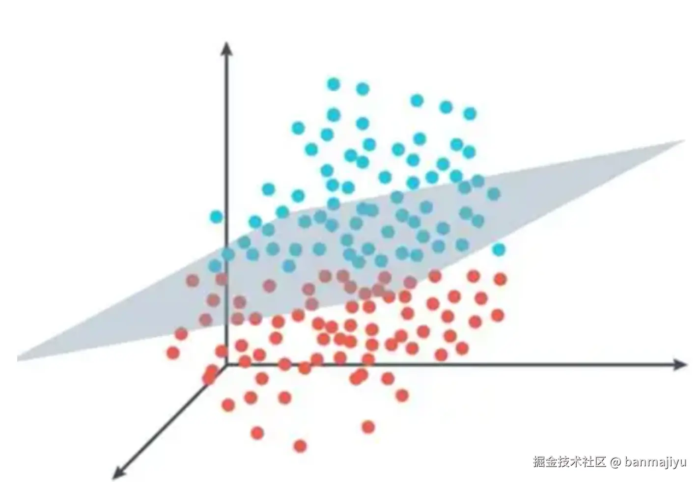
- 至少一个隐藏层：进行特征变换，把原始输入空间变换到另一个特征空间，使得在新空间中数据变得线性可分
- 输出层：产生最终预测

2. 为什么需要`MLP`？

刚才的实验完美展示了单层感知机的致命缺陷：无法解决线性不可分问题（如XOR）。MLP通过引入隐藏层和非线性激活函数，可以学习任意复杂的非线性决策边界。

二、MLP的数学原理

1. 网络结构

python 复制代码

输入层 (d维) → 隐藏层 (h维) → 输出层 (k维)
      x ∈ ℝ^d     h ∈ ℝ^h     y ∈ ℝ^k

2. 前向传播公式

对于两层MLP（一个隐藏层）：

第1层（输入→隐藏）：

python 复制代码

z[1] = W[1]·x + b[1]      # 线性变换
a[1] = σ(z[1])           # 非线性激活

第2层（隐藏→输出）：

python 复制代码

z[2] = W[2]·a[1] + b[2]    # 线性变换  
a[2] = σ(z[2])           # 输出激活

其中：

<math xmlns="http://www.w3.org/1998/Math/MathML"> W [ 1 ] ∈ R h × d , b [ 1 ] ∈ R h W[1] \in\mathbb{R}^{h\times d},b[1] \in \mathbb{R}^h </math>W[1]∈Rh×d,b[1]∈Rh：隐藏层参数
<math xmlns="http://www.w3.org/1998/Math/MathML"> W [ 2 ] ∈ R k × h , b [ 2 ] ∈ R k W[2] \in\mathbb{R}^{k\times h},b[2] \in \mathbb{R}^k </math>W[2]∈Rk×h,b[2]∈Rk：输出层参数
<math xmlns="http://www.w3.org/1998/Math/MathML"> σ \sigma </math>σ：激活函数（如ReLU、Sigmoid等）

3. 为什么能解决XOR问题？

几何解释：单层感知机只能画一条直线分割平面，而MLP可以画多条直线组合成曲线。
XOR的MLP解决方案（最小结构）：

python 复制代码

输入(2) → 隐藏层(2神经元) → 输出(1)
激活函数：ReLU
权重配置：
隐藏层：
  神经元1: w = [1, -1], b = -0.5  → 检测 x1=1且x2=0
  神经元2: w = [-1, 1], b = -0.5  → 检测 x1=0且x2=1
输出层：
  神经元: w = [1, 1], b = -1  → 组合隐藏层结果

三、核心组件

1. 激活函数（关键突破）

函数	公式	特点	适用场景
`ReLU`	<math xmlns="http://www.w3.org/1998/Math/MathML"> max ⁡ ( 0 , x ) \max(0, x) </math>max(0,x)	计算简单，缓解梯度消失	隐藏层默认选择
`Sigmoid`	<math xmlns="http://www.w3.org/1998/Math/MathML"> 1 1 + e − x \dfrac{1}{1+e⁻ˣ} </math>1+e−x1	输出 <math xmlns="http://www.w3.org/1998/Math/MathML"> ( 0 , 1 ) (0,1) </math>(0,1)，易饱和	二分类输出层
`Tanh`	<math xmlns="http://www.w3.org/1998/Math/MathML"> e x − e − x e x + e − x \dfrac{eˣ-e⁻ˣ}{eˣ+e⁻ˣ} </math>ex+e−xex−e−x	输出 <math xmlns="http://www.w3.org/1998/Math/MathML"> ( − 1 , 1 ) (-1,1) </math>(−1,1)，以 <math xmlns="http://www.w3.org/1998/Math/MathML"> 0 0 </math>0为中心	`RNN`隐藏层
`Leaky ReLU`	<math xmlns="http://www.w3.org/1998/Math/MathML"> max ⁡ ( α x , x ) \max(αx, x) </math>max(αx,x)	解决"死亡`ReLU`"	深度网络

激活函数的作用：
- 引入非线性 <math xmlns="http://www.w3.org/1998/Math/MathML"> → → </math>→ 使网络能拟合任意函数
- 决定信息如何传递 <math xmlns="http://www.w3.org/1998/Math/MathML"> → → </math>→ 不同的激活函数有不同的特性

2. 损失函数

任务类型	常用损失函数	公式
二分类	二元交叉熵	<math xmlns="http://www.w3.org/1998/Math/MathML"> L = − [ y ⋅ log ⁡ ( y ^ ) + ( 1 − y ) ⋅ log ⁡ ( 1 − y ^ ) ] L = -[y\cdot\log(\hat y) + (1-y)\cdot\log(1-\hat y)] </math>L=−[y⋅log(y^)+(1−y)⋅log(1−y^)]
多分类	交叉熵	<math xmlns="http://www.w3.org/1998/Math/MathML"> L = − ∑ y i ⋅ log ⁡ ( y ^ i ) L = -\sum y_i \cdot\log(\hat y_i) </math>L=−∑yi⋅log(y^i)
回归	均方误差	<math xmlns="http://www.w3.org/1998/Math/MathML"> L = 1 n ∑ ( y − y ^ i ) 2 L = \dfrac{1}{n}\sum(y-\hat y_i)^2 </math>L=n1∑(y−y^i)2

3. 反向传播算法

反向传播（Backpropagation）是MLP训练的核心：

python 复制代码

# 前向传播
z1 = W1·x + b1
a1 = σ(z1)
z2 = W2·a1 + b2
a2 = σ(z2)
loss = L(a2, y)

# 反向传播（链式法则）
dL/dz2 = dL/da2 * σ'(z2)      # 输出层梯度
dL/dW2 = dL/dz2 · a1ᵀ          # 输出层权重梯度
dL/db2 = dL/dz2               # 输出层偏置梯度

dL/dz1 = (W2ᵀ·dL/dz2) * σ'(z1) # 隐藏层梯度
dL/dW1 = dL/dz1 · xᵀ           # 隐藏层权重梯度
dL/db1 = dL/dz1               # 隐藏层偏置梯度

# 参数更新（梯度下降）
W1 = W1 - η·dL/dW1
b1 = b1 - η·dL/db1
W2 = W2 - η·dL/dW2  
b2 = b2 - η·dL/db2

四、MLP的Python实现

框架（纯手工，丑勿喷）：

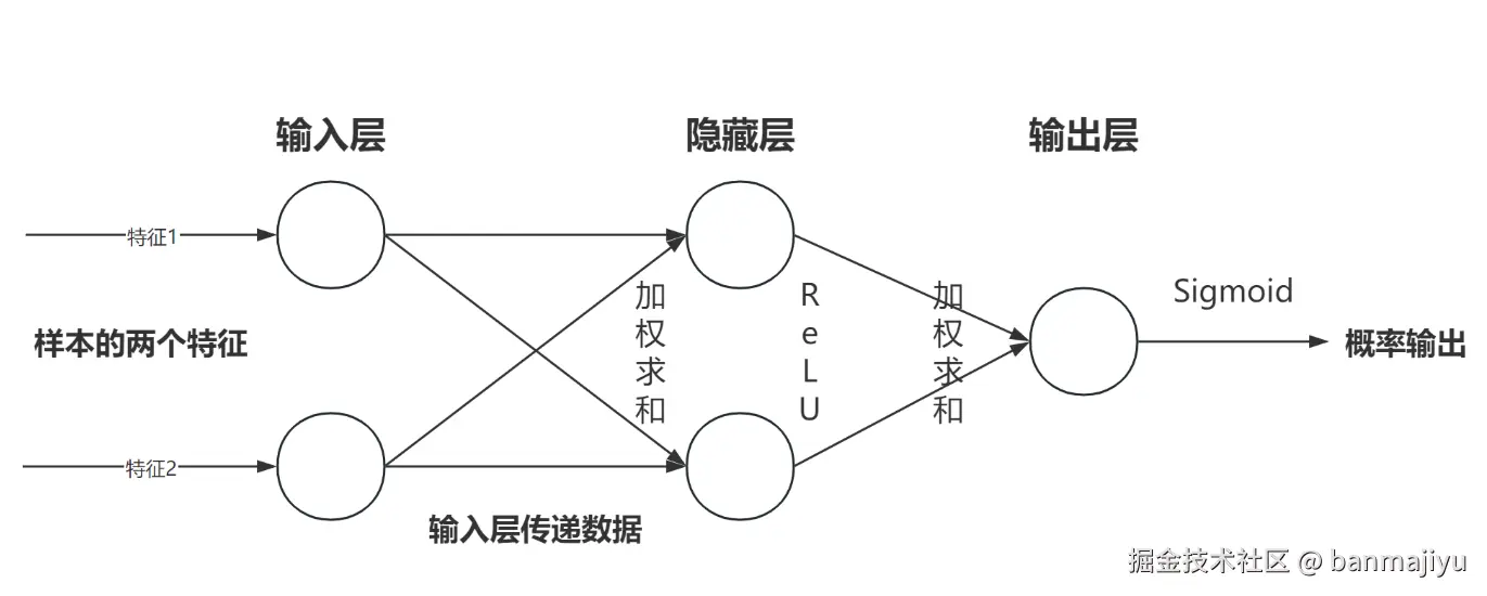
输入层 包含两个神经元，它们的功能是将数据直接传递给隐藏层神经元 ，由于XOR问题有两个输入数据（ <math xmlns="http://www.w3.org/1998/Math/MathML"> 2 2 </math>2个特征），所以需要两个输入层神经元。

隐藏层 也包含两个神经元，每个神经元相当于一个单层感知机 ，激活函数是ReLU。

输出层 包含一个神经元，激活函数是Sigmoid，作用是最终输出预测概率。

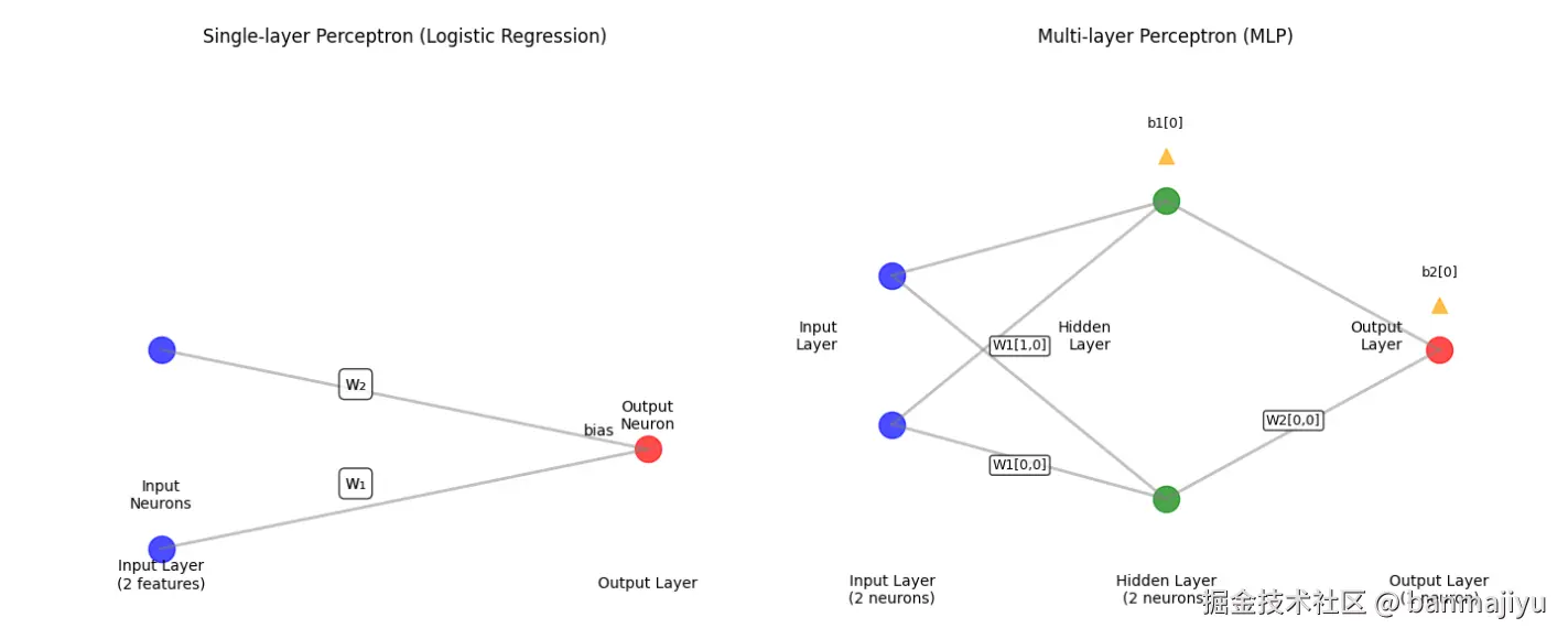
参数的作用是建立层与层之间的联系 。在单层感知机中，参数简单地连接了输入和输出，也就是说参数属于整个模型。而MLP中，输入层和输出层之间还有一个隐藏层，因此需要两组参数来分别连接输入层与隐藏层、隐藏层与输出层，参数属于层与层之间的连接，形成层级结构。

每个权重矩阵负责将前一层的输出转换为下一层的输入
<math xmlns="http://www.w3.org/1998/Math/MathML"> W 1 W_1 </math>W1将输入特征转换为隐藏层特征
<math xmlns="http://www.w3.org/1998/Math/MathML"> W 2 W_2 </math>W2将隐藏层特征转换为最终输出
这种设计允许网络学习多层特征表示

python 复制代码

import numpy as np

class MLP:
    def init(self, input_size, hidden_size, output_size, learning_rate=0.1):
        # 初始化参数
        self.W1 = np.random.randn(hidden_size, input_size) * 0.01   # 输入层到隐藏层的权重
        self.b1 = np.zeros((hidden_size, 1))                        # 输入层到隐藏层的偏置
        self.W2 = np.random.randn(output_size, hidden_size) * 0.01  # 隐藏层到输出层的权重
        self.b2 = np.zeros((output_size, 1))                        # 隐藏层到输出层的偏置
        self.lr = learning_rate                                     # 学习率
        
    def relu(self, x):  # ReLU激活函数，用于隐藏层
        return np.maximum(0, x)
    
    def relu_derivative(self, x):   # ReLU导数  
        return (x > 0).astype(float)
    
    def sigmoid(self, x):   # Sigmoid函数，用于输出层
        return 1 / (1 + np.exp(-x))
    
    def forward(self, X):                                       
        # 前向传播
        self.Z1 = np.dot(self.W1, X) + self.b1  # 隐藏层线性变换
        self.A1 = self.relu(self.Z1)    # 隐藏层激活
        self.Z2 = np.dot(self.W2, self.A1) + self.b2    # 输出层线性变换
        self.A2 = self.sigmoid(self.Z2) # 输出层激活
        return self.A2  # 返回输出层的激活值
    
    def backward(self, X, y, output):
        # 计算样本数
        m = X.shape[1]
        
        # 输出层梯度
        dZ2 = output - y    # 输出层误差
        dW2 = (1/m) * np.dot(dZ2, self.A1.T)    # 输出层权重梯度
        db2 = (1/m) * np.sum(dZ2, axis=1, keepdims=True)    # 输出层偏置梯度
        
        # 隐藏层梯度
        dA1 = np.dot(self.W2.T, dZ2)    # 输出层误差反向传播到隐藏层
        dZ1 = dA1 * self.relu_derivative(self.Z1)   # 隐藏层误差乘以ReLU导数
        dW1 = (1/m) * np.dot(dZ1, X.T)  # 隐藏层权重梯度
        db1 = (1/m) * np.sum(dZ1, axis=1, keepdims=True)    # 隐藏层偏置梯度
        
        # 更新参数
        self.W2 -= self.lr * dW2    # 更新隐藏层到输出层的权重
        self.b2 -= self.lr * db2    # 更新隐藏层到输出层的偏置
        self.W1 -= self.lr * dW1    # 更新输入层到隐藏层的权重
        self.b1 -= self.lr * db1    # 更新输入层到隐藏层的偏置
    
    def compute_loss(self, y, output):
        # 交叉熵损失
        m = y.shape[1]  # 样本数量
        loss = -(1/m) * np.sum(y * np.log(output) + (1-y) * np.log(1-output))
        return loss
    
    def train(self, X, y, epochs=10000):
        losses = []
        for epoch in range(epochs):
            # 前向传播
            output = self.forward(X)
            
            # 计算损失
            loss = self.compute_loss(y, output)
            losses.append(loss)
            
            # 反向传播，更新参数
            self.backward(X, y, output)
            
            if epoch % 1000 == 0:
                print(f"Epoch {epoch}, Loss: {loss:.6f}")
        
        return losses

# 测试XOR问题
def test_xor():
    # XOR数据
    X = np.array([[0, 0, 1, 1],
                  [0, 1, 0, 1]])  # 2×4
    y = np.array([[0, 1, 1, 0]])  # 1×4
    
    # 创建MLP：2输入 → 2隐藏神经元 → 1输出
    mlp = MLP(input_size=2, hidden_size=2, output_size=1, learning_rate=0.1)
    
    # 训练
    losses = mlp.train(X, y, epochs=10000)
    
    # 预测
    predictions = mlp.forward(X)
    print("\nXOR预测结果:")
    print(f"输入 (0,0): {predictions[0,0]:.4f} → 舍入: {round(predictions[0,0])}")
    print(f"输入 (0,1): {predictions[0,1]:.4f} → 舍入: {round(predictions[0,1])}")
    print(f"输入 (1,0): {predictions[0,2]:.4f} → 舍入: {round(predictions[0,2])}")
    print(f"输入 (1,1): {predictions[0,3]:.4f} → 舍入: {round(predictions[0,3])}")

if name == "main":
    test_xor()

训练结果：

python 复制代码

Epoch 0, Loss: 0.693131
Epoch 1000, Loss: 0.061531
Epoch 2000, Loss: 0.013892
Epoch 3000, Loss: 0.007434
Epoch 4000, Loss: 0.005013
Epoch 5000, Loss: 0.003756
Epoch 6000, Loss: 0.002995
Epoch 7000, Loss: 0.002485
Epoch 8000, Loss: 0.002121
Epoch 9000, Loss: 0.001847

XOR预测结果:
输入 (0,0): 0.0028 → 舍入: 0
输入 (0,1): 0.9995 → 舍入: 1
输入 (1,0): 0.9995 → 舍入: 1
输入 (1,1): 0.0028 → 舍入: 0

五、`MLP`的优缺点

优点

万能近似定理：单隐藏层MLP可近似任意连续函数
可解释性：相比CNN/RNN更易理解
灵活架构：可任意调整层数、神经元数
并行计算友好：全连接结构适合GPU加速

缺点

参数量爆炸：输入维度高时，参数量巨大（全连接）
容易过拟合：需要大量正则化技术
梯度问题：深层网络易梯度消失/爆炸
局部最优：非凸优化，易陷局部最小值

总结

XOR问题揭示了单层感知机的缺陷，也凸显了多层感知机的强大。然后没什么好总结的了......

预告：下一篇文章将聚焦MLP的应用......

异或问题（XOR Question）：从单层感知机到多层感知机