【论文总结】针对LoFTR在图像匹配中效率低下的问题,提出了Efficient LoFTR方法,通过两项核心技术创新实现了效率与精度的双重提升。首先,针对LoFTR在粗特征图上密集执行全局注意力导致的计算冗余问题,作者提出了聚合注意力机制(Aggregated Attention) ,该机制基于局部区域注意力信息相似性的观察,采用自适应token选择策略,仅对代表性token子集执行注意力计算,其他token通过聚合操作获取变换信息,将计算复杂度从 O ( N 2 ) O(N^2) O(N2)降低到 O ( M 2 ) O(M^2) O(M2)( M ≪ N M \ll N M≪N),显著减少了特征变换的计算成本。其次,针对LoFTR精细化阶段因对整个相关块进行期望计算而产生的空间方差问题,作者设计了两阶段相关层(Two-Stage Correlation Layer) :第一阶段通过互最近邻(MNN)匹配在精细特征块上准确定位像素级对应关系,过滤噪声响应;第二阶段仅在像素级匹配位置的微小邻域内进行局部相关性计算和期望操作,实现高精度的亚像素定位,同时避免远距离噪声的干扰。实验表明,该方法比LoFTR快约 2.5 2.5 2.5倍,甚至超越了稀疏匹配流程SuperPoint+LightGlue的效率,同时在多个任务上保持或超越了现有半密集匹配方法的精度,为大规模图像检索和三维重建等延迟敏感应用提供了高效可行的解决方案。
Abstract
We present a novel method for efficiently producing semidense matches across images. Previous detector-free matcher LoFTR has shown remarkable matching capability in handling large-viewpoint change and texture-poor scenarios but suffers from low efficiency. We revisit its design choices and derive multiple improvements for both efficiency and accuracy. One key observation is that performing the transformer over the entire feature map is redundant due to shared local information, therefore we propose an aggregated attention mechanism with adaptive token selection for efficiency. Furthermore, we find spatial variance exists in LoFTR's fine correlation module, which is adverse to matching accuracy. A novel two-stage correlation layer is proposed to achieve accurate subpixel correspondences for accuracy improvement. Our efficiency optimized model is ∼ 2.5 × \sim2.5\times ∼2.5× faster than LoFTR which can even surpass state-of-the-art efficient sparse matching pipeline SuperPoint + + + LightGlue. Moreover, extensive experiments show that our method can achieve higher accuracy compared with competitive semi-dense matchers, with considerable efficiency benefits. This opens up exciting prospects for large-scale or latency-sensitive applications such as image retrieval and 3 D 3D 3D reconstruction. Project page: https://github.com/zju3dv/efficientloftr.
【翻译】我们提出了一种新颖的方法,用于高效地生成图像间的半密集匹配。先前的无检测器匹配方法LoFTR在处理大视角变化和纹理贫乏场景方面展现了卓越的匹配能力,但存在效率低下的问题。我们重新审视了其设计选择,并在效率和精度两方面都得出了多项改进。一个关键观察是,由于局部信息的共享性,在整个特征图上执行transformer是冗余的,因此我们提出了一种带有自适应token选择的聚合注意力机制以提高效率。此外,我们发现LoFTR的精细相关模块中存在空间方差,这对匹配精度不利。我们提出了一种新颖的两阶段相关层,以实现精确的亚像素对应关系,从而提高精度。我们的效率优化模型比LoFTR快约 ∼ 2.5 × \sim2.5\times ∼2.5×倍,甚至可以超越最先进的高效稀疏匹配流程SuperPoint + + + LightGlue。此外,大量实验表明,与具有竞争力的半密集匹配器相比,我们的方法可以实现更高的精度,同时具有显著的效率优势。这为大规模或延迟敏感的应用(如图像检索和 3 D 3D 3D重建)开辟了令人兴奋的前景。
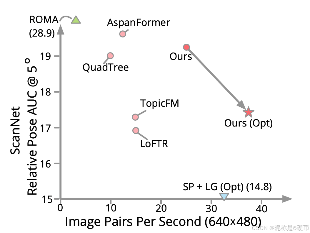
Figure 1. Matching Accuracy and Efficiency Comparisons. Our method achieves competitive accuracy compared with semi-dense matchers ( ◯ ) (\bigcirc) (◯) at a significantly higher speed. Compared with dense matcher ROMA ( △ ) (\triangle) (△) , our method is ∼ 7.5 × \sim7.5\times ∼7.5× faster. Moreover, our efficiency optimized model ( ⋆ ) (\star) (⋆) can surpass the robust sparse matching pipeline ( ▽ ) (\bigtriangledown) (▽) SuperPoint (SP) + LightGlue (LG) on efficiency with considerably better accuracy.
Image matching is the cornerstone of many 3D computer vision tasks, which aim to find a set of highly accurate correspondences given an image pair. The established matches between images have broad usages such as reconstructing the 3D world by structure from motion (SfM) 1, 21, 29, 47 or SLAM system 34, 35, and visual localization 42, 44, etc. Previous methods typically follow a two-stage pipeline: they first detect 41 and describe 53 a set of keypoints on each image, and then establish keypoint correspondences by handcrafted 31 or learning-based matchers 30, 43. These detector-based methods are efficient but suffer from robustly detecting repeatable keypoints across challenging pairs, such as extreme viewpoint changes and texture-poor regions.
Recently, LoFTR 50 introduces a detector-free matching paradigm with transformer to directly establish semi-dense correspondences between two images without detecting keypoints. With the help of the transformer mechanism to capture the global image context and the detector-free design, LoFTR shows a strong capability of matching challenging pairs, especially in texture-poor scenarios. To reduce the computation burden, LoFTR adopts a coarse-to-fine pipeline by first performing dense matching on downsampled coarse features maps, where transformer is applied. Then, the feature locations of coarse matches on one image are fixed, while their subpixel correspondences are searched on the other image by cropping feature patches based on coarse match, performing the feature correlation, and calculating expectation over the correlation patch.
Despite its impressive matching performance, LoFTR suffers from limited efficiency due to the large token size of performing transformer on the entire coarse feature map, which significantly barricades practical large-scale usages such as image retrieval 19 and SfM 47. A large bunch of LoFTR's follow-up works 7, 18, 36, 52, 59 have attempted to improve its matching accuracy. However, there are rare methods that focus on matching efficiency of detector-free matching. QuadTree Attention 52 incorporates multi-scale transformation with a gradually narrowed attention span to avoid performing attention on large feature maps. This strategy can reduce the computation cost, but it also divides a single coarse attention process into multiple steps, leading to increased latency.
【解析】LoFTR的效率瓶颈源于其在粗特征图层级的处理策略。在transformer架构中,计算复杂度与token数量的平方成正比,即 O ( N 2 ) O(N^2) O(N2)的复杂度,其中 N N N是token的数量。LoFTR在粗特征图上进行密集的全局注意力计算,即使特征图已经下采样到原图的 1 / 8 1/8 1/8分辨率,对于高分辨率输入图像而言,token数量仍然非常庞大。例如,对于一张 640 × 480 640\times480 640×480的图像,其 1 / 8 1/8 1/8下采样后的特征图尺寸为 80 × 60 80\times60 80×60,包含 4800 4800 4800个token,这导致自注意力和交叉注意力的计算量达到数千万次操作。这种计算负担在需要处理大量图像对的应用场景中(如大规模三维重建中的图像检索和匹配,或实时SLAM系统)成为严重的性能瓶颈。后续研究主要集中在提升匹配精度方面,通过引入更复杂的注意力机制、多尺度特征融合或更精细的匹配策略来改善匹配质量,但这些改进往往以增加计算复杂度为代价,进一步加剧了效率问题。QuadTree Attention尝试通过层次化的注意力机制来解决这个问题,其核心思想是在多个尺度上逐步缩小注意力的作用范围。具体而言,它首先在较粗的尺度上进行全局注意力计算以捕获大范围的对应关系,然后在更精细的尺度上将注意力限制在前一层确定的相关区域内。这种策略确实能够减少每一层的计算量,因为随着层级的深入,参与注意力计算的区域逐渐缩小。然而,这种分层处理方式引入了新的问题:原本可以在单次前向传播中完成的粗层级特征变换,现在被拆分成多个连续的处理阶段,每个阶段都需要独立的前向计算和中间结果的存储与传递,串行化的处理流程增加了模型的深度和数据流动的复杂性,导致实际推理时的延迟增加,特别是在GPU等并行计算设备上,这种串行依赖会降低硬件利用率。
In this paper, we revisit the design decisions of the detector-free matcher LoFTR, and propose a new matching algorithm that squeezes out redundant computations for significantly better efficiency while further improving the accuracy. As shown in Fig. 1, our approach achieves the best inference speed compared with recent image matching methods while being competitive in terms of accuracy. Our key innovations lie in introducing a token aggregation mechanism for efficient feature transformation and a two-stage correlation layer for correspondence refinement. Specifically, we find that densely performing global attention over the entire coarse feature map as in LoFTR is unnecessary, as the attention information is similar and shared in the local region. Therefore, we devise an aggregated attention mechanism to perform feature transformation on adaptively selected tokens, which is significantly compact and effectively reduces the cost of local feature transformation.
【解析】通过对注意力图的可视化和统计分析,作者发现在粗特征图上执行全局注意力时存在大量的信息冗余。这种冗余主要体现在空间局部性上:相邻位置的特征点在计算注意力时,其关注的区域和权重分布往往高度相似。这是因为图像的局部区域通常具有相似的语义内容和几何结构,导致这些位置的特征在进行全局上下文建模时会产生相近的注意力模式。基于这一观察,本文提出的token聚合机制采用了一种自适应的特征采样策略。该机制不是对特征图中的每个位置都独立计算注意力,而是首先识别出具有代表性的token子集。这个选择过程是自适应的,根据特征的显著性、多样性或其他学习到的准则来动态确定哪些token应该被保留用于注意力计算。被选中的token作为代表,通过注意力机制进行特征变换,而其他未被选中的token则通过聚合操作从这些代表token中获取变换后的信息。这种聚合可以是基于空间邻近性的插值,也可以是基于特征相似性的加权组合。通过这种方式,参与注意力计算的token数量大幅减少,从而将计算复杂度从 O ( N 2 ) O(N^2) O(N2)降低到 O ( M 2 ) O(M^2) O(M2),其中 M ≪ N M \ll N M≪N是聚合后的token数量。这种紧凑的表示不仅显著降低了计算成本,还保持了对全局上下文的建模能力,因为代表token的选择是基于整个特征图的信息。
In addition, we observe that there can be spatial variance in the matching refinement phase of LoFTR, which is caused by the expectation over the entire correlation patch when noisy feature correlation exists. To solve this issue, our approach designs a two-stage correlation layer that first locates pixel-level matches with the accurate mutual-nearestneighbor matching on fine feature patches, and then further refines matches for subpixel-level by performing the correlation and expectation locally within tiny patches.
【解析】LoFTR在精细化阶段的核心问题在于其对相关性图的处理方式。当系统在粗匹配阶段确定了一个初步的对应位置后,精细化模块会在该位置周围裁剪出一个特征块(通常是 5 × 5 5\times5 5×5或 7 × 7 7\times7 7×7的区域),然后计算这个块与目标图像对应区域之间的特征相关性,生成一个相关性图。LoFTR采用的策略是对整个相关性图进行softmax归一化后计算期望值,即对所有位置的坐标按其相关性分数进行加权平均,以此得到亚像素级的精确位置。这种全局期望计算的问题在于,当特征相关性中存在噪声时,即某些错误位置也具有较高的相关性分数时,这些噪声会参与到期望计算中,导致最终的亚像素位置估计产生偏差。这种偏差在空间上是不均匀的,取决于噪声的分布模式,因此称为空间方差。本文提出的两阶段相关层采用了更加稳健的策略来应对这个问题。第一阶段专注于像素级定位,采用互最近邻(Mutual Nearest Neighbor, MNN)匹配策略。MNN要求两个特征点互为对方的最近邻,即点 A A A在图像 I A I_A IA中找到图像 I B I_B IB中的最近邻点 B B B,同时点 B B B也必须找到点 A A A作为其最近邻。这种双向验证机制能够有效过滤掉大部分的错误匹配和噪声响应,因为噪声点很难同时满足双向最近邻的严格条件。通过MNN在精细特征块上进行匹配,系统能够准确地定位到整数像素位置的对应关系,这个位置虽然还不是最终的亚像素精度,但已经是一个高置信度的锚点。第二阶段在第一阶段确定的像素级位置基础上进行局部精细化。关键的改进在于,不再对整个相关块进行期望计算,而是仅在像素级匹配位置周围的一个非常小的邻域内(称为微小块,可能只有 3 × 3 3\times3 3×3甚至更小)进行相关性计算和期望操作。这种局部化策略基于一个合理的假设:既然第一阶段已经通过MNN确定了一个可靠的像素级位置,那么真实的亚像素位置应该就在这个位置的紧邻区域内。通过将期望计算限制在这个小范围内,远离真实位置的噪声响应被完全排除在外,不会对最终结果产生影响。同时,在这个小邻域内,相关性分数的分布通常更加平滑和可靠,因为这些位置在几何上非常接近,特征的一致性更高。这样计算出的期望值能够更准确地反映真实的亚像素偏移,从而实现高精度的对应关系定位。可以理解为:第一阶段通过MNN保证定位的可靠性,第二阶段通过局部精细化实现亚像素精度,同时避免噪声的干扰。
Extensive experiments are conducted on multiple tasks, including homography estimation, relative pose recovery, as well as visual localization, to show the efficacy of our method. Our pipeline pushes detector-free matching to unprecedented efficiency, which is ∼ 2.5 \sim2.5 ∼2.5 times faster than LoFTR and can even surpass the current state-of-the-art efficient sparse matcher LightGlue 30. Moreover, our framework can achieve comparable or even better matching accuracy compared with competitive detector-free baselines 7, 14, 15 with considerably higher efficiency.
In summary, this paper has the following contributions:
• A new detector-free matching pipeline with multiple improvements based on the comprehensive revisiting of LoFTR, which is significantly more efficient and with better accuracy.
• A novel aggregated attention network for efficient local feature transformation.
• A novel two-stage correlation refinement layer for accurate and subpixel-level refined correspondences.
Detector-Based Image Matching. Classical image matching methods 4, 31, 41 adopt handcrafted critics for detecting keypoints, describing and then matching them. Recent methods draw benefits from deep neural networks for both detection 24, 41, 46 and description 13, 33, 53, 54, where the robustness and discriminativeness of local descriptors are significantly improved. Besides, some methods 10, 12, 32, 38, 55 managed to learn the detector and descriptor together. SuperGlue 43 is a pioneering method that first introduces the transformer mechanism into matching, which has shown notable improvements over classical handcrafted matchers. As a side effect, it also costs more time, especially with many keypoints to match. To improve the efficiency, some subsequent works, such as 6, 48, endeavor to reduce the size of the attention mechanism, albeit at the cost of sacrificing performance. LightGlue 30 introduces a new scheme for efficient sparse matching that is adaptive to the matching difficulty, where the attention process can be stopped earlier for easy pairs. It is faster than SuperGlue and can achieve competitive performance. However, robustly detecting keypoints across images is still challenging, especially for texture-poor regions. Unlike them, our method focuses on the efficiency of the detector-free method, which eliminates the restriction of keypoint detection and shows superior performance for challenging pairs.
Detector-Free Image Matching. Detector-free methods directly match images instead of relying on a set of detected keypoints, producing semi-dense or dense matches. NCNet 39 represents all features and possible matches as a 4D correlation volume. Sparse NC-Net 40 utilizes sparse correlation layers to ease resolution limitations. Subsequently, DRC-Net 27 improves efficiency and further improves performance in a coarse-to-fine manner.
LoFTR 50 first employs the Transformer in detectorfree matching to model the long-range dependencies. It shows remarkable matching capabilities, however, suffers from low efficiency due to the huge computation of densely transforming entire coarse feature maps. Many followup works further improve the matching accuracy. Matchformer 59 and AspanFormer 7 perform attention on multiscale features, where local attention regions of 7 are found with the help of estimated flow. QuadTree 52 gradually restricts the attention span during hierarchical attention to relevant areas, which can reduce overall computation. However, these designs contribute marginally or even decrease efficiency, since the hierarchical nature of multi-scale attention will further introduce latencies. TopicFM 18 first assigns features with similar semantic meanings to the same topic, where attention is conducted within each topic for efficiency. Since it needs to sequentially process each token's features for transformation, the efficiency improvement is limited. Moreover, performing local attention within topics can potentially restrict the capability of modeling long-range dependencies. Compared with them, the proposed aggregated attention module in our method significantly improves efficiency while achieving better accuracy.
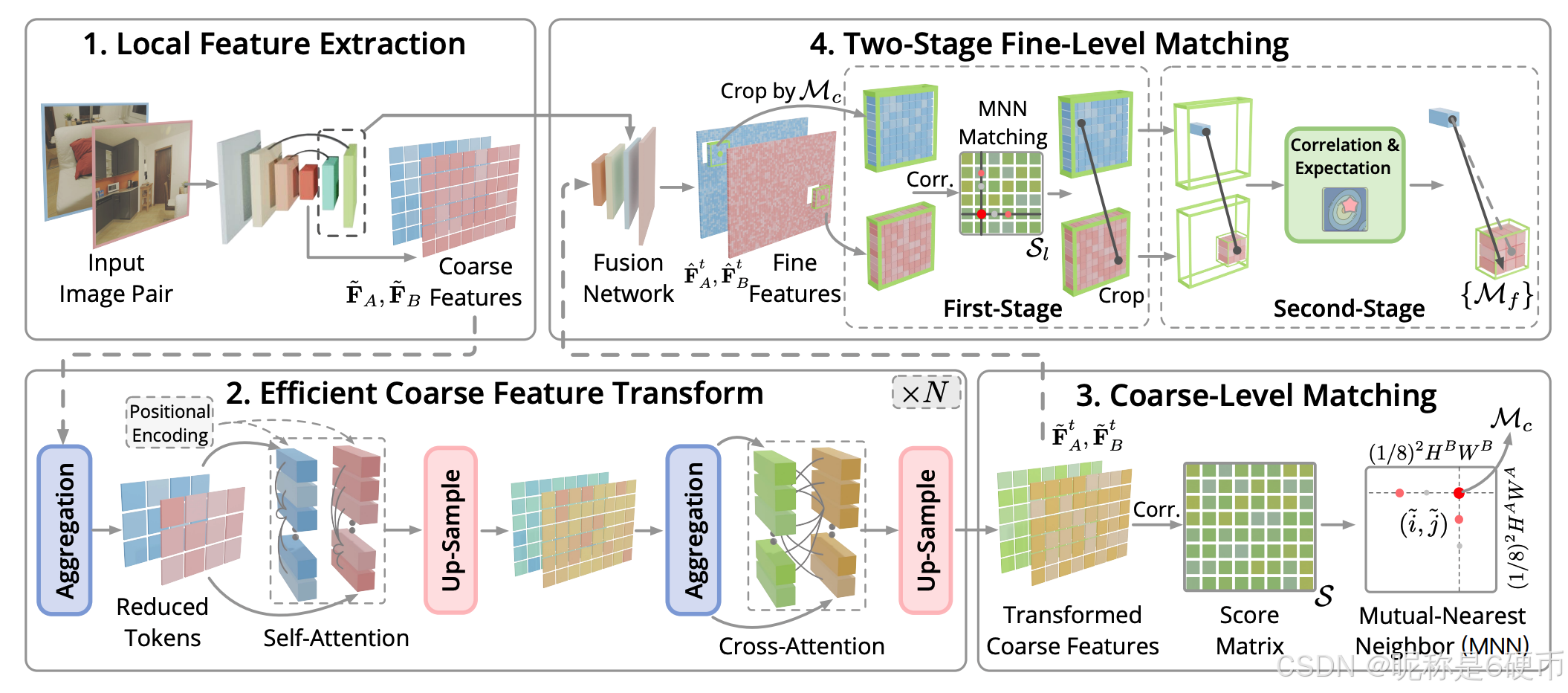
Figure 2. Pipeline Overview. (1) Given an image pair, a CNN network extracts coarse feature maps F ~ A \tilde{\mathbf{F}}{A} F~A and F ~ B \tilde{\mathbf{F}}{B} F~B , as well as fine features. (2) Then, we transform coarse features for more discriminative feature maps by interleaving our aggregated self- and cross-attention N N N times, where adaptively feature aggregation is performed to reduce token size before each attention for efficiency. (3) Transformed coarse features are correlated for the score matrix S S S . Mutual-nearest-neighbor (MNN) searching is followed to establish coarse matches { M c } \{\mathcal{M}{c}\} {Mc} . (4) To refine coarse matches, discriminative fine features F ^ A t \hat{\mathbf{F}}{A}^{t} F^At , F ^ B t \hat{\mathbf{F}}{B}^{t} F^Bt in full resolution are obtained by fusing transformed coarse features F ~ A t \tilde{\mathbf{F}}{A}^{t} F~At , F ~ B t \tilde{\mathbf{F}}{B}^{t} F~Bt with backbone features. Feature patches are then cropped centered at each coarse match M c \mathcal{M}{c} Mc . A two-stage refinement is followed to obtain sub-pixel correspondence M f \mathcal{M}_{f} Mf .
【翻译】图2. 流程概览。(1) 给定一对图像,CNN网络提取粗特征图 F ~ A \tilde{\mathbf{F}}{A} F~A和 F ~ B \tilde{\mathbf{F}}{B} F~B,以及精细特征。(2) 然后,我们通过交替进行聚合自注意力和交叉注意力 N N N次来变换粗特征以获得更具判别性的特征图,其中在每次注意力之前自适应地执行特征聚合以减少token大小从而提高效率。(3) 变换后的粗特征被用于计算相关性以得到分数矩阵 S S S。随后进行互最近邻(MNN)搜索以建立粗匹配 { M c } \{\mathcal{M}{c}\} {Mc}。(4) 为了精细化粗匹配,通过将变换后的粗特征 F ~ A t \tilde{\mathbf{F}}{A}^{t} F~At、 F ~ B t \tilde{\mathbf{F}}{B}^{t} F~Bt与骨干网络特征融合,获得全分辨率的判别性精细特征 F ^ A t \hat{\mathbf{F}}{A}^{t} F^At、 F ^ B t \hat{\mathbf{F}}{B}^{t} F^Bt。然后以每个粗匹配 M c \mathcal{M}{c} Mc为中心裁剪特征块。随后进行两阶段精细化以获得亚像素对应关系 M f \mathcal{M}_{f} Mf。
【解析】整个流程可以分为四个主要阶段。第一阶段是特征提取,系统接收一对输入图像后,通过卷积神经网络骨干提取多尺度的特征表示。这里提取的特征包括两个层级:粗特征图 F ~ A \tilde{\mathbf{F}}{A} F~A和 F ~ B \tilde{\mathbf{F}}{B} F~B通常是原图 1 / 8 1/8 1/8分辨率的下采样特征,用于后续的全局匹配;精细特征则保持更高的分辨率(如 1 / 4 1/4 1/4或 1 / 2 1/2 1/2),用于最终的精确定位。粗特征负责建立全局对应关系,精细特征负责局部精确化。第二阶段是高效的特征变换,这是作者的核心创新之一。系统对提取的粗特征进行 N N N次迭代的注意力变换,每次迭代都交替执行自注意力和交叉注意力操作。自注意力使得每张图像内部的特征能够相互交互,捕获图像内的上下文信息和长程依赖关系;交叉注意力则让两张图像的特征相互关联,使得系统能够学习到跨图像的对应模式。关键的效率改进在于,在每次注意力计算之前,系统会自适应地执行特征聚合操作,将大量的token压缩成更少的代表性token。这种聚合不是简单的下采样,而是根据特征的显著性和代表性进行智能选择,既保留了关键信息,又大幅减少了参与注意力计算的token数量,从而将计算复杂度从 O ( N 2 ) O(N^2) O(N2)降低到 O ( M 2 ) O(M^2) O(M2),其中 M ≪ N M \ll N M≪N。经过多次迭代后,粗特征被变换成更具判别性的表示,能够更准确地区分不同的图像区域。第三阶段是粗匹配的建立,系统计算变换后的粗特征之间的相关性,生成一个分数矩阵 S S S。这个矩阵的每个元素 S i j S_{ij} Sij表示图像 A A A中位置 i i i的特征与图像 B B B中位置 j j j的特征之间的相似度或匹配置信度。基于这个分数矩阵,系统采用互最近邻搜索策略来建立初步的粗匹配集合 { M c } \{\mathcal{M}{c}\} {Mc}。互最近邻要求双向验证:如果图像 A A A中的点 i i i在图像 B B B中找到最近邻点 j j j,同时点 j j j也必须将点 i i i作为其最近邻,这种双向约束能够有效过滤掉大量的错误匹配,提高匹配的可靠性。此时得到的匹配是在粗特征图分辨率下的整数像素位置,精度还不够高。第四阶段是精细化匹配,这是另一个核心创新。系统首先通过融合变换后的粗特征 F ~ A t \tilde{\mathbf{F}}{A}^{t} F~At、 F ~ B t \tilde{\mathbf{F}}{B}^{t} F~Bt与骨干网络提取的原始特征,生成全分辨率的判别性精细特征 F ^ A t \hat{\mathbf{F}}{A}^{t} F^At、 F ^ B t \hat{\mathbf{F}}{B}^{t} F^Bt。这种融合结合了粗特征的全局语义信息和精细特征的局部细节信息,使得最终的特征既具有判别性又保持高分辨率。对于粗匹配集合中的每一对匹配点 M c \mathcal{M}{c} Mc,系统以该点为中心在精细特征图上裁剪出一个局部特征块。然后执行两阶段精细化过程:第一阶段通过互最近邻匹配在精细特征块上定位像素级的准确位置,第二阶段在该位置的极小邻域内进行局部相关性计算和期望操作,得到亚像素级的精确偏移。这种两阶段设计既保证了定位的可靠性(通过第一阶段的MNN),又实现了高精度(通过第二阶段的局部精细化),同时避免了噪声的干扰。最终输出的 M f \mathcal{M}_{f} Mf是一组亚像素精度的对应关系,可以直接用于下游任务如位姿估计、三维重建等。
Dense matching methods 14, 15, 56 are designed to estimate all possible correspondences between two images, which show strong robustness. However, they are generally much slower compared with sparse and semi-dense methods. Unlike them, our method produces semi-dense matches with competitive performance and considerably better efficiency.
【解析】密集匹配方法的核心思想是为图像中的每一个像素或几乎每一个像素都寻找其在另一幅图像中的对应位置,从而建立一个完整的、逐像素级别的对应关系映射。这种全面的匹配策略带来了显著的优势:由于考虑了图像中的所有位置,系统能够在纹理贫乏、重复模式、大视角变化等困难场景下依然保持较高的匹配成功率。密集匹配不依赖于特定的关键点检测,因此不会因为检测失败而丢失重要的对应关系,这使得它在处理低纹理区域(如墙面、天空)或存在运动模糊的图像时表现出色。然而,这种全面性是以巨大的计算代价为前提的。对于一幅分辨率为 H × W H \times W H×W的图像,密集匹配需要为 H × W H \times W H×W个位置中的每一个都计算其与另一幅图像中所有可能位置的相似度,这导致计算复杂度达到 O ( H 2 W 2 ) O(H^2W^2) O(H2W2)的量级。即使采用各种优化策略,密集匹配的运行时间仍然远超稀疏方法和半密集方法。稀疏匹配方法只关注图像中的少量关键点(通常几百到几千个),因此计算量大幅减少,但可能在关键点检测失败的区域无法建立对应关系。半密集方法则在两者之间取得平衡,它不像密集方法那样处理每一个像素,而是选择性地在图像的重要区域或具有足够纹理信息的区域建立对应关系,从而在保持较高匹配覆盖率的同时控制计算成本。本文提出的方法属于半密集匹配范畴,通过精心设计的特征聚合和注意力机制,在匹配数量和质量上达到了与密集方法相当的水平,但运行效率却接近甚至超过了一些稀疏方法。
Transformer has been broadly used in multiple vision tasks, including feature matching. The efficiency and memory footprint of handling large token sizes are the main limitations of transformer 58, where some methods 22, 23, 60 attempt to reduce the complexity to a linear scale to alleviate these problems. Some methods 9, 26 propose optimizing transformer models for specific hardware architectures for memory and running-time efficiency. They are orthogonal to our method and can be naturally adapted into the pipeline for further efficiency improvement.
Given a pair of images I A , I B \mathbf{I}{A},\mathbf{I}{B} IA,IB , our objective is to establish a set of reliable correspondences between them. We achieve this by a coarse-to-fine matching pipeline, which first establishes coarse matches on downsampled feature maps and then refines them for high accuracy. An overview of our pipeline is shown in Fig. 2.
【翻译】给定一对图像 I A , I B \mathbf{I}{A},\mathbf{I}{B} IA,IB,我们的目标是在它们之间建立一组可靠的对应关系。我们通过粗到精的匹配流程来实现这一目标,该流程首先在下采样的特征图上建立粗匹配,然后对其进行精细化以获得高精度。我们流程的概览如图2所示。
Image feature maps are first extracted by a lightweight backbone for later transformation and matching. Unlike LoFTR and many other detector-free matchers that use a heavy multibranch ResNet 20 network for feature extraction, we alternate to a lightweight single-branch network with reparameterization 11 to achieve better inference efficiency while preserving the model performance.
In particular, a multi-branch CNN network with residual connections is applied during training for maximum representational power. At inference time, we losslessly convert the feature backbone into an efficient single-branch network by adopting the reparameterization technique 11, which is achieved by fusing parallel convolution kernels into a single one. Then, the intermediate 1 / 8 1/8 1/8 down-sampled coarse features F ~ A \tilde{\mathbf{F}}{A} F~A , F ~ B \tilde{\mathbf{F}}{B} F~B and fine features in 1 / 4 1/4 1/4 and 1 / 2 1/2 1/2 resolutions are extracted efficiently for later coarse-to-fine matching.
【翻译】具体而言,在训练期间应用带有残差连接的多分支CNN网络以获得最大的表示能力。在推理时,我们通过采用重参数化技术11将特征骨干网络无损地转换为高效的单分支网络,这是通过将并行卷积核融合为单个卷积核来实现的。然后,高效地提取中间的 1 / 8 1/8 1/8下采样粗特征 F ~ A \tilde{\mathbf{F}}{A} F~A、 F ~ B \tilde{\mathbf{F}}{B} F~B以及 1 / 4 1/4 1/4和 1 / 2 1/2 1/2分辨率的精细特征,用于后续的粗到精匹配。
【解析】在训练阶段,网络采用多分支CNN架构并配备残差连接。残差连接通过引入跳跃连接将输入直接加到输出上,形成 y = F ( x ) + x y = F(x) + x y=F(x)+x的结构,其中 F ( x ) F(x) F(x)是卷积层学习的残差映射,有两个关键优势:一是缓解了深层网络的梯度消失问题,使得梯度可以通过跳跃连接直接反向传播到浅层,从而支持更深的网络训练;二是让网络更容易学习恒等映射,如果某一层的最优映射接近恒等变换,网络只需将 F ( x ) F(x) F(x)学习为接近零的函数即可。多分支结构结合残差连接,使得训练阶段的网络具有极强的表示能力,能够学习到复杂的特征变换。当训练完成进入推理阶段时,重参数化技术发挥作用。假设多分支结构中有 k k k个并行的卷积分支,每个分支的卷积核为 W 1 , W 2 , . . . , W k W_1, W_2, ..., W_k W1,W2,...,Wk,对于输入 x x x,多分支的输出是 ∑ i = 1 k W i ∗ x \sum_{i=1}^{k} W_i * x ∑i=1kWi∗x。由于卷积操作的线性性质,这等价于 ( ∑ i = 1 k W i ) ∗ x (\sum_{i=1}^{k} W_i) * x (∑i=1kWi)∗x,也就是说,我们可以将所有并行卷积核直接相加得到一个等效的单一卷积核 W f u s e d = ∑ i = 1 k W i W_{fused} = \sum_{i=1}^{k} W_i Wfused=∑i=1kWi。这个融合过程是完全无损的,融合后的单分支网络与原多分支网络在数学上完全等价,但结构大大简化。在推理时,系统只需要用这个融合后的卷积核进行一次卷积操作,而不是分别计算 k k k个分支再求和,这显著减少了计算量和内存访问次数。特征提取的输出包含多个尺度的特征图。粗特征 F ~ A \tilde{\mathbf{F}}{A} F~A和 F ~ B \tilde{\mathbf{F}}{B} F~B是原始图像 1 / 8 1/8 1/8分辨率的下采样特征,这个尺度的特征具有较大的感受野,能够捕获全局的语义信息和上下文关系,适合用于建立初步的全局对应关系。同时,系统还提取 1 / 4 1/4 1/4和 1 / 2 1/2 1/2分辨率的精细特征,这些特征保留了更多的空间细节信息,虽然感受野相对较小,但能够提供更精确的位置信息。
3.2. Efficient Local Feature Transformation(高效局部特征变换)
After the feature extraction, the coarse-level feature maps F ~ A \tilde{\mathbf{F}}{A} F~A and F ~ B \tilde{\mathbf{F}}{B} F~B are transformed by interleaving self- and crossattention n n n times to improve discriminativeness.(We feed feature of one image as query and feature of the other image
as key and value into cross-attention, similar to SG 43and LoFTR 50.) The transformed features are denoted as F ~ A t , F ~ B t \tilde{\mathbf{F}}{A}^{t},\tilde{\mathbf{F}}{B}^{t} F~At,F~Bt .
【翻译】在特征提取之后,粗级别特征图 F ~ A \tilde{\mathbf{F}}{A} F~A和 F ~ B \tilde{\mathbf{F}}{B} F~B通过交替进行自注意力和交叉注意力 n n n次来变换以提高判别性。(我们将一幅图像的特征作为查询,另一幅图像的特征作为键和值输入到交叉注意力中,类似于SG 43和LoFTR 50。)变换后的特征表示为 F ~ A t , F ~ B t \tilde{\mathbf{F}}{A}^{t},\tilde{\mathbf{F}}{B}^{t} F~At,F~Bt。
【解析】特征提取完成后,系统需要对粗级别特征图进行深度变换以增强其判别能力。这个变换过程采用交替执行自注意力和交叉注意力的策略,重复 n n n次迭代。自注意力机制作用于单张图像内部,让特征图中的每个位置都能与同一图像中的其他所有位置进行信息交互,从而捕获图像内部的长程依赖关系和上下文信息。这种内部交互使得每个特征点不再是孤立的局部描述子,而是融合了全局语义信息的表示。交叉注意力则建立两幅图像之间的关联,具体实现时将图像A的特征作为查询 Q Q Q,图像B的特征同时作为键 K K K和值 V V V输入到注意力模块。这样图像A中的每个特征点都会查询图像B中所有位置的特征,计算相似度权重后对图像B的特征进行加权聚合,使得图像A的特征能够感知到图像B中与之相关的区域信息。反向操作同样进行,图像B的特征也会查询图像A。这种双向的跨图像注意力让两幅图像的特征相互增强,网络能够学习到哪些区域在两幅图像中是对应的,从而为后续的匹配提供更具判别性的特征表示。经过 n n n次自注意力和交叉注意力的交替迭代,原始的粗特征 F ~ A \tilde{\mathbf{F}}{A} F~A和 F ~ B \tilde{\mathbf{F}}{B} F~B被逐步变换为更加丰富和判别性更强的特征表示 F ~ A t \tilde{\mathbf{F}}{A}^{t} F~At和 F ~ B t \tilde{\mathbf{F}}{B}^{t} F~Bt,其中上标 t t t表示经过变换后的特征。这些变换后的特征不仅包含了原始的局部外观信息,还融合了图像内部的全局上下文以及跨图像的对应关系线索。
Previous methods often perform attention on the entire coarse-level feature maps, where linear attention instead of vanilla attention is applied to ensure a manageable computation cost. However, the efficiency is still limited due to the large token size of coarse features. Moreover, the usage of linear attention leads to sub-optimal model capability. Unlike them, we propose efficient aggregated attention for both efficiency and performance.
【解析】当处理高分辨率图像时,即使是下采样到 1 / 8 1/8 1/8分辨率的粗特征图,token数量仍然可能达到数千甚至上万,导致二次方的计算量变得难以承受。为了缓解这个问题,现有方法通常采用线性注意力机制,通过引入核函数近似 ϕ ( ⋅ ) \phi(\cdot) ϕ(⋅)将计算复杂度从 O ( N 2 ) O(N^2) O(N2)降低到 O ( N ) O(N) O(N)。线性注意力通过改变计算顺序,先计算 ϕ ( K ) T ϕ ( V ) \phi(K)^T\phi(V) ϕ(K)Tϕ(V)得到一个固定大小的矩阵,再与 ϕ ( Q ) \phi(Q) ϕ(Q)相乘,避免了显式构建完整的注意力矩阵。然而这种近似带来两个问题:首先,尽管复杂度降为线性,但当token数量 N N N本身很大时,线性复杂度 O ( N ) O(N) O(N)的计算量仍然相当可观,效率提升有限;其次,线性注意力通过核函数近似softmax操作,这种近似会损失标准注意力的表达能力,导致模型无法充分捕获复杂的特征关系,最终影响匹配精度。本文提出的聚合注意力机制从根本上解决这个矛盾,通过在注意力计算之前对特征进行智能聚合,将token数量从 N N N大幅减少到 M M M(其中 M ≪ N M \ll N M≪N),然后在这些聚合后的token上应用标准的注意力机制。这样既保持了标准注意力的完整表达能力,又因为token数量的大幅减少使得二次方复杂度 O ( M 2 ) O(M^2) O(M2)在实际中变得可行,实现了效率和性能的双重提升。
Preliminaries. First, we provide a brief overview of the commonly used vanilla attention and linear attention. Vanilla attention is a core mechanism in transformer encoder layer, relying on three inputs: query Q, key K, and value V. The resultant output is a weighted sum of the value, where the weighted matrix is determined by the query and its corresponding key. Formally, the attention function is defined as follows:
V a n i l l a A t t e n t i o n ( Q , K , V ) = s o f t m a x ( Q K T ) V . \mathrm{VanillaAttention}(Q,K,V)=\mathrm{softmax}(Q K^{T})V. VanillaAttention(Q,K,V)=softmax(QKT)V.
However, applying the vanilla attention directly to dense local features is impractical due to the significant token size. To address this issue, previous methods use linear attention to reduce the computational complexity from quadratic to linear:
L i n e a r A t t e n t i o n ( Q , K , V ) = ϕ ( Q ) ( ϕ ( K ) T ϕ ( V ) ) . \mathrm{LinearAttention}(Q,K,V)=\phi(Q)(\phi(K)^{T}\phi(V)). LinearAttention(Q,K,V)=ϕ(Q)(ϕ(K)Tϕ(V)).
where ϕ ( ⋅ ) = e l u ( ⋅ ) + 1 \phi(\cdot)=e l u(\cdot)+1 ϕ(⋅)=elu(⋅)+1 . However, it comes at the cost of reduced representational power, which is also observed by 5.
【翻译】预备知识。首先,我们简要概述常用的标准注意力和线性注意力。标准注意力是transformer编码器层的核心机制,依赖于三个输入:查询Q、键K和值V。输出结果是值的加权和,其中权重矩阵由查询及其对应的键决定。形式上,注意力函数定义如下:然而,由于token规模较大,直接将标准注意力应用于密集局部特征是不切实际的。为了解决这个问题,以往的方法使用线性注意力将计算复杂度从二次方降低到线性:其中 ϕ ( ⋅ ) = e l u ( ⋅ ) + 1 \phi(\cdot)=e l u(\cdot)+1 ϕ(⋅)=elu(⋅)+1。然而,这是以降低表示能力为代价的,这一点在5中也有观察到。
【解析】标准注意力机制是transformer架构的基础组件,其工作原理建立在查询-键-值三元组的交互之上。给定查询矩阵 Q ∈ R N × d Q \in \mathbb{R}^{N \times d} Q∈RN×d、键矩阵 K ∈ R M × d K \in \mathbb{R}^{M \times d} K∈RM×d和值矩阵 V ∈ R M × d V \in \mathbb{R}^{M \times d} V∈RM×d,其中 N N N和 M M M分别表示查询和键值对的token数量, d d d表示特征维度。标准注意力首先计算查询与所有键之间的相似度,通过矩阵乘法 Q K T QK^T QKT得到一个 N × M N \times M N×M的注意力得分矩阵,该矩阵的每个元素 ( i , j ) (i,j) (i,j)表示第 i i i个查询与第 j j j个键的匹配程度。随后对每一行应用softmax归一化,将得分转换为概率分布,确保每个查询对所有键的注意力权重之和为1。最终输出通过这些归一化权重对值矩阵进行加权求和得到,使得每个查询位置的输出特征是所有值特征的加权组合,权重反映了查询与各个键的相关性强度。动态地聚合全局信息,让每个位置都能根据其与其他位置的语义关联来调整自身的特征表示。然而标准注意力的计算瓶颈在于注意力矩阵 Q K T QK^T QKT的构建和softmax操作,其时间复杂度为 O ( N × M × d + N × M 2 ) O(N \times M \times d + N \times M^2) O(N×M×d+N×M2),空间复杂度为 O ( N × M ) O(N \times M) O(N×M)。当处理密集特征图时,token数量 N N N和 M M M可能达到数千甚至数万级别,导致二次方的计算和内存开销变得难以承受。线性注意力通过引入核函数 ϕ ( ⋅ ) \phi(\cdot) ϕ(⋅)对查询、键进行非线性变换,然后利用矩阵乘法的结合律改变计算顺序。具体而言,标准注意力可以写成 softmax ( Q K T ) V \text{softmax}(QK^T)V softmax(QKT)V,而线性注意力通过核近似将softmax替换为 ϕ ( Q ) ϕ ( K ) T \phi(Q)\phi(K)^T ϕ(Q)ϕ(K)T,然后先计算 ϕ ( K ) T ϕ ( V ) \phi(K)^T\phi(V) ϕ(K)Tϕ(V)得到一个 d × d d \times d d×d的矩阵,再与 ϕ ( Q ) \phi(Q) ϕ(Q)相乘。由于 d d d通常远小于 N N N和 M M M,这种重排将复杂度降低到 O ( N × d 2 + M × d 2 ) O(N \times d^2 + M \times d^2) O(N×d2+M×d2),实现了线性复杂度。本文采用的核函数 ϕ ( x ) = elu ( x ) + 1 \phi(x) = \text{elu}(x) + 1 ϕ(x)=elu(x)+1保证了输出的非负性,其中 elu \text{elu} elu是指数线性单元激活函数。尽管线性注意力大幅提升了计算效率,但其代价是表示能力的下降。核函数近似无法完全捕捉softmax的归一化特性和尖锐的注意力分布,导致模型难以精确地将注意力集中在最相关的少数位置上,而是倾向于产生更平滑、更分散的注意力权重。这种表示能力的削弱在需要精细匹配的任务中尤为明显,因为匹配质量高度依赖于注意力机制能否准确识别和强化真正的对应关系。文献5的实验观察也证实了这一现象,说明线性注意力在效率和性能之间存在固有的权衡。
Aggragated Attention Module. After comprehensively investigating the mechanism of the transformer on coarse feature maps, we have two observations that motivate us to devise a new efficient aggregated attention. First, the attention regions of neighboring query tokens are similar, thus we can aggregate the neighboring tokens of f i f_{i} fi to prevent the redundant computation. Second, most of the attention weights of each query token are concentrated on a small number of key tokens, hence we can select the salient tokens of f j f_{j} fj before attention to reduce the computation.
【翻译】聚合注意力模块。在全面研究了transformer在粗特征图上的机制后,我们有两个观察结果促使我们设计一种新的高效聚合注意力。首先,相邻查询token的注意力区域是相似的,因此我们可以聚合 f i f_{i} fi的相邻token以防止冗余计算。其次,每个查询token的大部分注意力权重集中在少数几个关键token上,因此我们可以在注意力计算之前选择 f j f_{j} fj的显著token以减少计算量。
【解析】通过对transformer在粗特征图上的工作机制进行深入分析,作者发现了两个关键的统计规律。第一个观察是空间局部性原理:在特征图中,空间位置相邻的查询token往往对应于图像中相邻的像素或区域,这些相邻区域在视觉内容上通常具有较高的相关性。当这些相邻的查询token分别计算注意力时,它们所关注的键token区域呈现出高度的重叠性。如果对每个查询token都独立执行完整的注意力计算,就会产生大量的重复计算。因此,可以将 f i f_i fi中空间相邻的多个查询token聚合成一个代表性token,用这个聚合token来代表整个局部区域进行注意力计算,从而避免对相似注意力模式的重复计算。第二个观察揭示了注意力权重的稀疏性特征:在标准注意力机制中,每个查询token理论上会与所有键token计算相似度并分配权重,但实际分析发现,经过softmax归一化后的注意力权重分布呈现显著的长尾特征。绝大部分权重值集中在少数几个键token上,而其余大量键token的权重接近于零。这些权重极小的键token对最终的加权求和结果贡献微乎其微,但在计算过程中仍然需要参与矩阵运算,造成计算资源的浪费。因此,可以在注意力计算之前对 f j f_j fj进行预筛选,只保留那些显著的、可能获得高注意力权重的键token,从而大幅减少参与注意力计算的token数量。
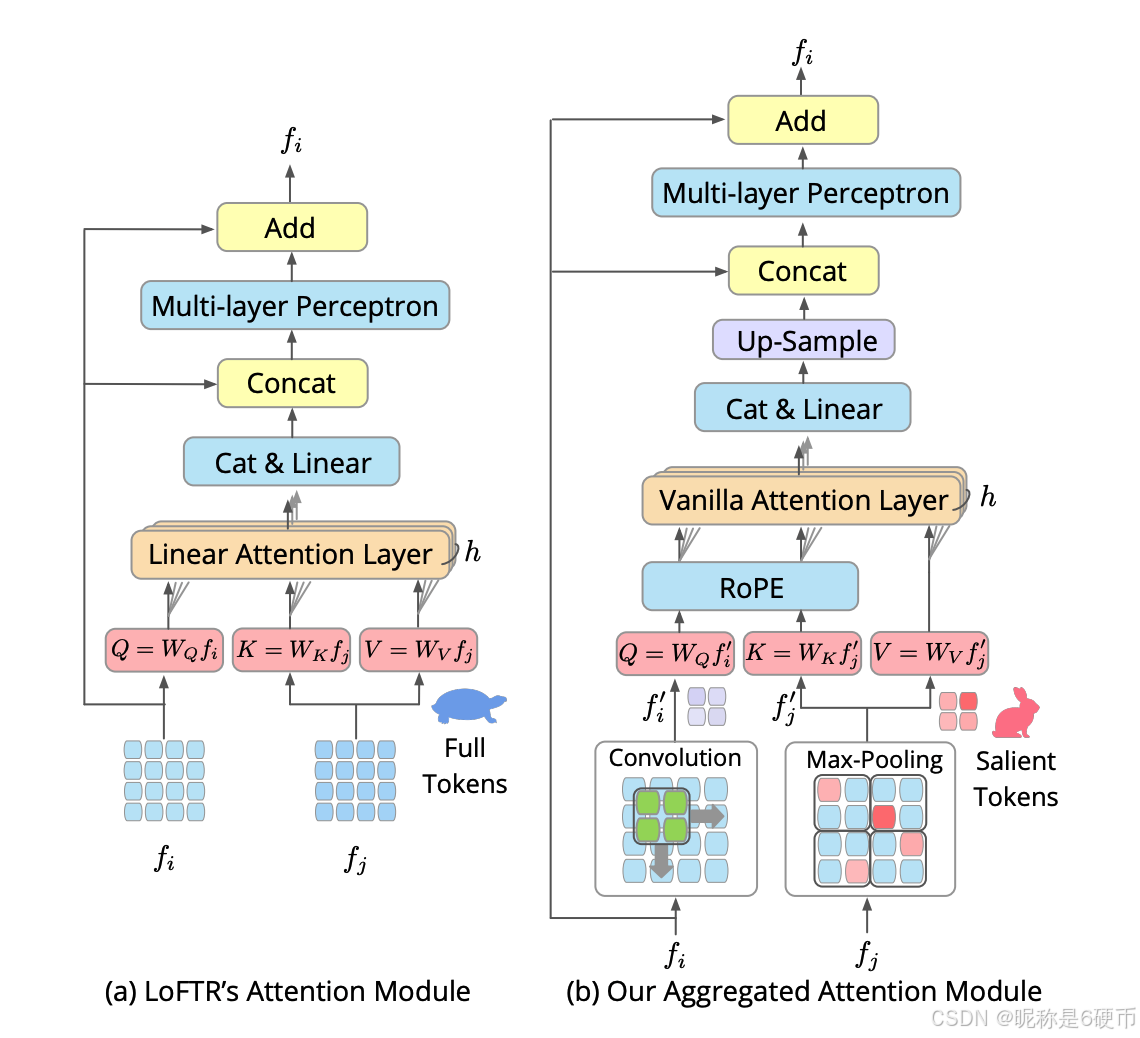
Figure 3. Detailed Transformer Module Comparison. Unlike LoFTR which uses all tokens of feature maps to compute attention and resort to linear attention to reduce the computational cost, the proposed attention module first aggregates features for salient tokens, which is significantly more efficient for attention. Then the vanilla attention is utilized to transform aggregated features, where relative positional encoding is inserted to capture the spatial information. Transformed features are upsampled and fused with the original features to form the final features.
Therefore, we propose to first aggregate the f i f_{i} fi token utilizing a depth-wise convolution network, and f j f_{j} fj is aggregated by a max pooling layer to get reduced salient tokens:
f i ′ = C o n v 2 D ( f i ) , f j ′ = M a x P o o l ( f j ) , f_{i}^{\prime}=\mathrm{Conv2D}(f_{i}),f_{j}^{\prime}=\mathrm{MaxPool}(f_{j}), fi′=Conv2D(fi),fj′=MaxPool(fj),
where Conv2D is implemented by a strided depthwise convolution with a kernel size of s × s s\times s s×s , identical to that of the max-pooling layer. Then positional encoding and vanilla attention are followed to process reduced tokens. Positional encoding (PE) can help to model the spatial location contexts, where RoPE 49 is adopted in practice to account for more robust relative positions, inspired by 30. Note that the PE layer is enabled exclusively for self-attention and skipped during cross-attention. The transformed feature map is then upsampled and fused with f i f_{i} fi for the final feature map. Due to the aggregation and selection, the number of tokens in f i ′ f_{i}^{\prime} fi′ and f j ′ f_{j}^{\prime} fj′ is reduced by s 2 s^{2} s2 , which contributes to the efficiency of the attention phase.
【翻译】因此,我们提出首先利用深度卷积网络聚合 f i f_{i} fi的token,并通过最大池化层聚合 f j f_{j} fj以获得精简的显著token:其中Conv2D由步长为 s × s s\times s s×s的深度可分离卷积实现,与最大池化层的核大小相同。然后使用位置编码和标准注意力来处理精简后的token。位置编码(PE)可以帮助建模空间位置上下文,实践中采用RoPE 49来考虑更鲁棒的相对位置,受30启发。注意,PE层仅在自注意力中启用,在交叉注意力期间跳过。然后将变换后的特征图上采样并与 f i f_{i} fi融合以形成最终特征图。由于聚合和选择, f i ′ f_{i}^{\prime} fi′和 f j ′ f_{j}^{\prime} fj′中的token数量减少了 s 2 s^{2} s2倍,这有助于提高注意力阶段的效率。
【解析】针对前述两个观察结果,作者设计聚合策略来同时处理查询特征 f i f_i fi和键值特征 f j f_j fj。对于查询特征 f i f_i fi的聚合,采用深度可分离卷积网络来实现。深度可分离卷积将标准卷积分解为逐通道卷积和逐点卷积两个步骤,在保持特征提取能力的同时大幅降低参数量和计算量。这里使用步长为 s s s、卷积核大小为 s × s s \times s s×s的深度卷积,其作用是在空间维度上对相邻的token进行聚合。由于步长为 s s s,卷积操作在滑动时会跳过 s − 1 s-1 s−1个位置,这样输出特征图的空间尺寸会缩小为原来的 1 / s 1/s 1/s,实现了token数量的减少。深度卷积的优势在于它能够在聚合过程中保留局部空间结构信息,通过卷积核的权重学习来自适应地融合相邻token的特征,使得聚合后的token能够有效代表原始局部区域的语义信息。对于键值特征 f j f_j fj的聚合,则采用最大池化操作。最大池化层同样使用 s × s s \times s s×s的窗口大小和 s s s的步长,确保与深度卷积的下采样率保持一致。最大池化的工作原理是在每个 s × s s \times s s×s的局部窗口内选择响应值最大的特征,因为响应值较大的特征通常对应于更具判别性和信息量的区域。通过最大池化,系统能够筛选出 f j f_j fj中最显著的token,过滤掉那些响应较弱、对匹配贡献较小的token。经过聚合操作后,得到精简的特征 f i ′ f_i' fi′和 f j ′ f_j' fj′,它们的token数量相比原始特征减少了 s 2 s^2 s2倍。在这些精简的token上应用标准注意力机制,计算复杂度从原来的 O ( N 2 ) O(N^2) O(N2)降低到 O ( ( N / s 2 ) 2 ) = O ( N 2 / s 4 ) O((N/s^2)^2) = O(N^2/s^4) O((N/s2)2)=O(N2/s4),实现了显著的效率提升。在注意力计算之前,系统引入位置编码来为token注入空间位置信息。采用旋转位置编码RoPE,是一种相对位置编码方案,它通过旋转变换将相对位置信息编码到查询和键的向量中,使得注意力得分能够隐式地反映token之间的相对空间距离。RoPE相比绝对位置编码具有更好的外推性和对相对位置关系的建模能力。需要注意的是,位置编码仅在自注意力阶段使用,而在交叉注意力阶段被跳过。这是因为自注意力处理单张图像内部的token关系,空间位置信息对于理解图像内部结构至关重要;而交叉注意力建立两幅图像之间的对应关系,两幅图像的绝对空间位置没有直接的对应关系,因此不需要位置编码。经过标准注意力变换后,得到的特征图需要恢复到原始分辨率。系统通过上采样操作将变换后的特征图从 1 / s 1/s 1/s分辨率恢复到原始分辨率,然后与输入的 f i f_i fi进行融合。这种融合采用残差连接的思想,将变换后的特征与原始特征相加或拼接,既保留了原始特征中的细节信息,又融入了经过全局注意力增强后的语义信息,形成最终的输出特征图。整个聚合注意力模块通过智能的token精简策略,在保持标准注意力完整表达能力的同时,将计算复杂度降低了 s 4 s^4 s4倍,实现了效率和性能的平衡。
3.3. Coarse-level Matching Module(粗级别匹配模块)
We establish coarse-level matches based on the previously transformed coarse feature maps F ~ A t , F ~ B t \tilde{\mathbf{F}}{A}^{t},\tilde{\mathbf{F}}{B}^{t} F~At,F~Bt . Coarse correspondences indicate rough match regions for later subpixel-level matching in the refinement phase. To achieve this, F ~ A t \tilde{\mathbf{F}}{A}^{t} F~At and F ~ B t \tilde{\mathbf{F}}{B}^{t} F~Bt are densely correlated to build a score matrix S S S . The softmax operator on both S S S dimensions (referred to as dualsoftmax) is then applied to obtain the probability of mutual nearest matching, which is commonly used in 39, 50, 57. The coarse correspondences { M c } \{\mathcal{M}_{c}\} {Mc} are established by selecting matches above the score threshold τ \tau τ while satisfying the mutual-nearest-neighbor (MNN) constraint.
【翻译】我们基于先前变换后的粗特征图 F ~ A t , F ~ B t \tilde{\mathbf{F}}{A}^{t},\tilde{\mathbf{F}}{B}^{t} F~At,F~Bt建立粗级别匹配。粗对应关系指示了后续精细化阶段中亚像素级匹配的粗略匹配区域。为了实现这一点, F ~ A t \tilde{\mathbf{F}}{A}^{t} F~At和 F ~ B t \tilde{\mathbf{F}}{B}^{t} F~Bt被密集地关联以构建得分矩阵 S S S。然后在 S S S的两个维度上应用softmax算子(称为双softmax)以获得互最近邻匹配的概率,这在39, 50, 57中被普遍使用。粗对应关系 { M c } \{\mathcal{M}_{c}\} {Mc}通过选择得分高于阈值 τ \tau τ且满足互最近邻(MNN)约束的匹配来建立。
【解析】粗级别匹配模块在经过transformer交互后的粗特征图 F ~ A t \tilde{\mathbf{F}}{A}^{t} F~At和 F ~ B t \tilde{\mathbf{F}}{B}^{t} F~Bt之间建立初步对应关系,为后续精细化阶段提供搜索范围约束。具体流程:首先计算密集相关性,对图像A中每个位置 i i i和图像B中每个位置 j j j计算特征向量内积相似度,形成得分矩阵 S ∈ R H c W c × H c W c S \in \mathbb{R}^{H_c W_c \times H_c W_c} S∈RHcWc×HcWc。然后应用双向softmax归一化:先对矩阵每一行应用softmax使图像A中每个点对图像B所有点的得分归一化为概率分布,再对每一列应用softmax使图像B中每个点对图像A所有点的得分也归一化。这种双向归一化确保了匹配的互相性,有效抑制了一对多或多对一的错误匹配。最后通过阈值筛选和互最近邻约束建立粗对应关系 { M c } \{\mathcal{M}_{c}\} {Mc}:只保留得分高于阈值 τ \tau τ且满足互最近邻条件的匹配对,即位置 i i i在图像B中的最佳匹配是 j j j,同时 j j j在图像A中的最佳匹配也是 i i i。这种双重约束机制能够有效过滤掉大量的错误匹配,确保粗对应关系的可靠性。
Efficient Inference Strategy. We observe that the dualsoftmax operator in the coarse matching can significantly restrict the efficiency in inference due to the large token size, especially for high-resolution images. Moreover, we find that the dual-softmax operator is crucial for training, dropping it at inference time while directly using the score matrix S S S for MNN matching can also work well with better efficiency.
【翻译】高效推理策略。我们观察到粗匹配中的双softmax算子由于较大的token规模会显著限制推理效率,特别是对于高分辨率图像。此外,我们发现双softmax算子对于训练至关重要,但在推理时去掉它而直接使用得分矩阵 S S S进行MNN匹配也能很好地工作,且效率更高。
The reason for using the dual-softmax operator in training is that it can help to train discriminative features. Intuitively, with the softmax operation, the matching score between two pixels can also conditioned on other pixels. This mechanism forces the network to improve feature similarity of true correspondences while suppressing similarity with irrelevant points. With trained discriminative features, the softmax operation can be potentially eliminated during inference.
We denote the model skipping dual-softmax layer in inference as efficiency optimized model. Results in Tab. 1 demonstrate the effectiveness of this design.
As overviewed in Fig. 2 (4), with established coarse matches { M c } \{\mathcal{M}{c}\} {Mc} , we refine them for sub-pixel accuracy with our refinement module. It is composed of an efficient feature patch extractor for discriminative fine features, followed by a twostage feature correlation layer for final matches { M f } \{\mathcal{M}{f}\} {Mf} .
【翻译】如图2(4)所示,在建立了粗匹配 { M c } \{\mathcal{M}{c}\} {Mc}之后,我们通过精细化模块将其精炼到亚像素精度。该模块由一个用于判别性精细特征的高效特征块提取器组成,随后是一个两阶段特征相关层以获得最终匹配 { M f } \{\mathcal{M}{f}\} {Mf}。
Efficient Fine Feature Extraction. We first extract discriminative fine feature patches centered at each coarse match M c \mathcal{M}{c} Mc by an efficient fusion network for later match refinement. For efficiency, our key idea here is to re-leverage the previously transformed coarse features F ~ A t \tilde{\mathbf{F}}{A}^{t} F~At , F ~ B t \tilde{\mathbf{F}}_{B}^{t} F~Bt to obtain cross-view attended discriminative fine features, instead of introducing additional feature transform networks as in LoFTR 50.
【翻译】高效精细特征提取。我们首先通过一个高效融合网络提取以每个粗匹配 M c \mathcal{M}{c} Mc为中心的判别性精细特征块,用于后续的匹配精炼。为了提高效率,我们的关键思想是重新利用先前变换后的粗特征 F ~ A t \tilde{\mathbf{F}}{A}^{t} F~At、 F ~ B t \tilde{\mathbf{F}}_{B}^{t} F~Bt来获得跨视图注意的判别性精细特征,而不是像LoFTR 50那样引入额外的特征变换网络。
【解析】传统方法如LoFTR需要为精细匹配阶段单独构建特征变换网络,这会引入额外的计算开销和参数量,作者认为:在粗匹配阶段经过多层transformer交互后得到的粗特征 F ~ A t \tilde{\mathbf{F}}{A}^{t} F~At和 F ~ B t \tilde{\mathbf{F}}{B}^{t} F~Bt已经包含了丰富的跨视图上下文信息和判别性语义。这些特征经过自注意力增强了单视图内的特征一致性,经过交叉注意力建立了两视图间的语义对应关系,因此具有很强的判别能力。与其重新构建特征提取网络,不如直接复用这些已经过充分交互的粗特征,通过轻量级的融合网络将其上采样到原始图像分辨率,从而获得既具有判别性又包含跨视图注意信息的精细特征。这种特征复用策略避免了重复的特征变换计算,降低了模型的计算复杂度和参数量,同时保持了特征的判别能力。
To be specific, F ~ A t \tilde{\mathbf{F}}{A}^{t} F~At and F ~ B t \tilde{\mathbf{F}}{B}^{t} F~Bt are adaptively fused with 1 / 4 1/4 1/4 and 1 / 2 1/2 1/2 resolution backbone features by convolution and upsampling to obtain fine feature maps F ^ A t , F ^ B t \hat{\mathbf{F}}{A}^{t},\hat{\mathbf{F}}{B}^{t} F^At,F^Bt in the original image resolution. Then local feature patches are cropped on fine feature maps centered at each coarse match. Since only shallow feed-forward networks are included, our fine feature fusion network is remarkably efficient.
【翻译】具体来说, F ~ A t \tilde{\mathbf{F}}{A}^{t} F~At和 F ~ B t \tilde{\mathbf{F}}{B}^{t} F~Bt通过卷积和上采样与 1 / 4 1/4 1/4和 1 / 2 1/2 1/2分辨率的骨干特征自适应融合,以获得原始图像分辨率的精细特征图 F ^ A t , F ^ B t \hat{\mathbf{F}}{A}^{t},\hat{\mathbf{F}}{B}^{t} F^At,F^Bt。然后在精细特征图上以每个粗匹配为中心裁剪局部特征块。由于只包含浅层前馈网络,我们的精细特征融合网络非常高效。
【解析】精细特征的生成采用多尺度特征融合策略。骨干网络在特征提取过程中会产生不同分辨率的中间特征,其中 1 / 4 1/4 1/4分辨率特征保留了较多的空间细节信息, 1 / 2 1/2 1/2分辨率特征则在细节和语义之间取得平衡。将经过transformer交互的粗特征 F ~ A t \tilde{\mathbf{F}}{A}^{t} F~At和 F ~ B t \tilde{\mathbf{F}}{B}^{t} F~Bt与这些多尺度骨干特征进行自适应融合,可以同时利用粗特征中的全局上下文和跨视图对应信息,以及骨干特征中的局部细节信息。融合过程通过卷积操作实现特征通道的自适应加权组合,通过上采样操作将特征分辨率逐步恢复到原始图像尺寸,最终得到精细特征图 F ^ A t \hat{\mathbf{F}}{A}^{t} F^At和 F ^ B t \hat{\mathbf{F}}{B}^{t} F^Bt。在这些精细特征图上,系统以每个粗匹配位置为中心裁剪出局部特征块,这些特征块的空间范围限定了后续精细匹配的搜索区域,避免了全局搜索的巨大计算开销。整个融合网络只使用浅层的前馈卷积层,没有引入复杂的注意力机制或深层网络结构,因此计算效率极高,能够快速生成高质量的精细特征用于后续的亚像素级匹配。
Two-Stage Correlation for Refinement. Based on the extracted fine local feature patches of coarse matches, we search for high-accurate sub-pixel matches. To refine a coarse match, a commonly used strategy 7, 18, 50 is to select the center-patch feature of I A {\mathbf{I}}_{A} IA as a fixed reference point, and perform feature correlation and expectation on the entire corresponding feature patch for its fine match. However, this refinement-by-expectations will introduce location variance to the final match, because irrelevant regions also have weights and can affect results. Therefore, we propose a novel two-stage correlation module to solve this problem.
【翻译】用于精细化的两阶段相关性。基于提取的粗匹配的精细局部特征块,我们搜索高精度的亚像素匹配。为了精炼粗匹配,一种常用策略7, 18, 50是选择 I A {\mathbf{I}}_{A} IA的中心块特征作为固定参考点,并在整个对应特征块上执行特征相关性和期望计算以获得其精细匹配。然而,这种基于期望的精细化会给最终匹配引入位置方差,因为不相关区域也有权重并可能影响结果。因此,我们提出了一种新颖的两阶段相关性模块来解决这个问题。
Our idea is to utilize a mutual-nearest-neighbor (MNN) matching to get intermediate pixel-level refined matches in the first stage, and then refine them for subpixel accuracy by correlation and expectation. Motivations are that MNN matching don't have spatial variance since matches are selected by directly indexing pixels with maximum scores, but cannot achieve sub-pixel accuracy. Conversely, refinementby-expectation can achieve sub-pixel accuracy but variance exists. The proposed two-stage refinement can draw benefits by combining the best of both worlds.
Specifically, to refine a coarse-level correspondence M c \mathcal{M}{c} Mc , the first-stage refinement phase densely correlates their fine feature patches to obtain the local patch score matrix S l \boldsymbol{S{l}} Sl . MNN searching is then applied on S l \boldsymbol{S_{l}} Sl to get intermediate pixel-level fine matches. To limit the overall match number, we select the top-1 fine match for one coarse match by sorting the correlation scores.
【翻译】具体来说,为了精炼一个粗级别对应关系 M c \mathcal{M}{c} Mc,第一阶段精细化阶段密集地关联它们的精细特征块以获得局部块得分矩阵 S l \boldsymbol{S{l}} Sl。然后在 S l \boldsymbol{S_{l}} Sl上应用MNN搜索以获得中间像素级精细匹配。为了限制总体匹配数量,我们通过对相关性得分排序为一个粗匹配选择top-1精细匹配。
【解析】第一阶段的具体实现流程如下:对于每个粗匹配 M c \mathcal{M}{c} Mc,系统已经提取了图像A和图像B中对应位置周围的局部精细特征块。这些特征块的尺寸通常为 w × w w \times w w×w像素,包含了粗匹配点周围的局部上下文信息。系统对这两个特征块进行密集相关性计算,即计算图像A特征块中每个位置与图像B特征块中每个位置之间的特征相似度,形成局部得分矩阵 S l ∈ R w × w × w × w \boldsymbol{S{l}} \in \mathbb{R}^{w \times w \times w \times w} Sl∈Rw×w×w×w。然后在这个得分矩阵上执行互最近邻搜索:对于图像A特征块中的每个位置,找到其在图像B特征块中得分最高的对应位置;同时对于图像B特征块中的每个位置,找到其在图像A特征块中得分最高的对应位置。只有当两个位置互为最近邻时,才认为它们构成有效匹配。由于一个粗匹配可能在其局部区域内产生多个满足MNN条件的像素级匹配候选,为了控制最终输出的匹配数量并选择最可靠的结果,系统对所有候选匹配按相关性得分排序,只保留得分最高的top-1匹配作为该粗匹配的像素级精细化结果。这样既保证了匹配质量,又避免了冗余匹配的产生。
Then, we further refine these pixel-level matches for subpixel accuracy by our second-stage refinement. Since the matching accuracy has already significantly improved in first-stage refinement, now we can use a tiny local window for correlation and expectation with a maximum suppression of location variance. In practice, we correlate the feature of each point in I A \mathbf{I}{A} IA with a 3 × 3 3\times3 3×3 feature patch centered at its fine match in I B \mathbf{I}{B} IB . The softmax operator is then applied to get a match distribution matrix and the final refined match is obtained by calculating expectations.
【翻译】然后,我们通过第二阶段精细化进一步将这些像素级匹配精炼到亚像素精度。由于匹配精度在第一阶段精细化中已经显著提高,现在我们可以使用一个很小的局部窗口进行相关性和期望计算,最大程度地抑制位置方差。在实践中,我们将 I A \mathbf{I}{A} IA中每个点的特征与以其在 I B \mathbf{I}{B} IB中的精细匹配为中心的 3 × 3 3\times3 3×3特征块进行关联。然后应用softmax算子以获得匹配分布矩阵,并通过计算期望获得最终精炼匹配。
The entire pipeline is trained end-to-end by supervising the coarse and refinement matching modules separately.
【翻译】整个流程通过分别监督粗匹配和精细化匹配模块进行端到端训练。
Coarse-Level Matching Supervision. The coarse ground truth matches { M c } g t \{\mathcal{M}{c}\}{g t} {Mc}gt with a total number of N N N are built by warping grid-level points from I A \mathbf{I}{A} IA to I B {\bf{I}}{B} IB via depth maps and image poses following previous methods 43, 50. The produced correlation score matrix s s s in coarse matching is supervised by minimizing the log-likelihood loss over locations of { M c } g t \{\mathcal{M}{c}\}{g t} {Mc}gt :
L c = − 1 N ∑ ( i ~ , j ~ ) ∈ { M c } g t log S ( i ~ , j ~ ) . \begin{array}{r}{\mathcal{L}{c}=-\frac{1}{N}\sum{(\tilde{i},\tilde{j})\in\{\mathcal{M}{c}\}{g t}}\log S\left(\tilde{i},\tilde{j}\right).}\end{array} Lc=−N1∑(i~,j~)∈{Mc}gtlogS(i~,j~).
【翻译】粗级别匹配监督。粗粒度真值匹配 { M c } g t \{\mathcal{M}{c}\}{g t} {Mc}gt总共有 N N N个,通过深度图和图像位姿将网格级点从 I A \mathbf{I}{A} IA变换到 I B {\bf{I}}{B} IB来构建,遵循先前方法43, 50。粗匹配中产生的相关性得分矩阵 s s s通过最小化 { M c } g t \{\mathcal{M}{c}\}{g t} {Mc}gt位置上的对数似然损失来监督。
【解析】粗匹配的监督需要首先构建真值匹配对。由于训练数据集提供了每张图像的深度图和相机位姿,可以利用这些几何信息建立像素级的对应关系。具体过程是在图像A的粗特征图上均匀采样网格点,对于每个网格点,利用其对应原图位置的深度值将其反投影到三维空间,然后利用两个相机之间的相对位姿关系将该三维点投影到图像B中,得到其在图像B中的对应位置。这个过程称为几何变换或warping。通过这种方式可以为每个采样点建立准确的真值对应关系,形成粗匹配真值集合 { M c } g t \{\mathcal{M}{c}\}{g t} {Mc}gt,包含 N N N对匹配。网络在粗匹配阶段会输出相关性得分矩阵 S S S,其中每个元素 S ( i ~ , j ~ ) S(\tilde{i},\tilde{j}) S(i~,j~)表示图像A中位置 i ~ \tilde{i} i~与图像B中位置 j ~ \tilde{j} j~匹配的概率。损失函数 L c \mathcal{L}_{c} Lc采用负对数似然形式,对所有真值匹配对的得分取对数并求平均。这个损失函数的作用是鼓励网络为真值匹配对分配高概率,即让 S ( i ~ , j ~ ) S(\tilde{i},\tilde{j}) S(i~,j~)接近1。由于得分矩阵经过softmax归一化,提高真值位置的得分必然会降低其他位置的得分,从而实现对正确匹配的强化和对错误匹配的抑制。负对数似然损失在概率预测任务中广泛使用,因为它直接优化预测分布与真实分布之间的交叉熵,具有良好的梯度性质和收敛特性。
Fine-Level Matching Supervision. We train the proposed two-stage fine-level matching module by separately supervising the two phases. The first stage fine loss L f 1 \mathcal{L}{f1} Lf1 is to minimize the log-likelihood loss of each fine local score matrix S l \boldsymbol{S{l}} Sl based on the pixel-level ground truth fine matches, similar to coarse loss. The second stage is trained by L f 2 \mathcal{L}{f2} Lf2 that calculates the ℓ 2 \ell{2} ℓ2 loss between the final subpixel matches { M f } \{\mathcal{M}{f}\} {Mf} and ground truth fine matches { M f } g t \{\mathcal{M}{f}\}_{g t} {Mf}gt .
【翻译】精细级别匹配监督。我们通过分别监督两个阶段来训练所提出的两阶段精细级别匹配模块。第一阶段精细损失 L f 1 \mathcal{L}{f1} Lf1是基于像素级真值精细匹配最小化每个精细局部得分矩阵 S l \boldsymbol{S{l}} Sl的对数似然损失,类似于粗损失。第二阶段通过 L f 2 \mathcal{L}{f2} Lf2训练,该损失计算最终亚像素匹配 { M f } \{\mathcal{M}{f}\} {Mf}与真值精细匹配 { M f } g t \{\mathcal{M}{f}\}{g t} {Mf}gt之间的 ℓ 2 \ell_{2} ℓ2损失。
【解析】精细化模块的两阶段设计对应两种不同的监督策略。第一阶段执行互最近邻匹配,输出离散的像素级匹配位置,其监督方式与粗匹配类似。对于每个粗匹配,系统会在其周围的局部特征块上计算密集相关性得分矩阵 S l \boldsymbol{S_{l}} Sl。利用深度图和位姿信息可以计算出精确到像素级的真值匹配位置,第一阶段损失 L f 1 \mathcal{L}{f1} Lf1就是对这些局部得分矩阵应用负对数似然损失,鼓励网络在正确的像素位置产生高得分。这个损失的形式与粗匹配损失相同,但作用在更高分辨率的精细特征上,引导网络学习局部判别性特征以实现精确的像素级定位。第二阶段执行亚像素精炼,通过期望计算输出连续坐标,其监督方式需要改变。由于输出是连续的亚像素坐标而非离散概率分布,这里采用 ℓ 2 \ell{2} ℓ2损失即欧氏距离损失。 L f 2 \mathcal{L}{f2} Lf2计算网络预测的最终亚像素匹配位置 { M f } \{\mathcal{M}{f}\} {Mf}与真值位置 { M f } g t \{\mathcal{M}{f}\}{g t} {Mf}gt之间的平方距离,直接惩罚位置偏差。这种回归式的损失函数适合优化连续输出,能够引导网络在像素级匹配的基础上进行微调,将匹配精度推向亚像素级别。两阶段分别使用分类式损失和回归式损失,与各自的输出形式和优化目标相匹配,确保了精细化模块的有效训练。
The total loss is the weighted sum of all supervisions: L = L c + α L f 1 + β L f 2 \mathcal{L}=\mathcal{L}{c}+\alpha\mathcal{L}{f1}+\beta\mathcal{L}_{f2} L=Lc+αLf1+βLf2 .
【翻译】总损失是所有监督的加权和: L = L c + α L f 1 + β L f 2 \mathcal{L}=\mathcal{L}{c}+\alpha\mathcal{L}{f1}+\beta\mathcal{L}_{f2} L=Lc+αLf1+βLf2。
【解析】整个网络的优化目标是三个损失项的加权组合。粗匹配损失 L c \mathcal{L}{c} Lc、第一阶段精细损失 L f 1 \mathcal{L}{f1} Lf1和第二阶段精细损失 L f 2 \mathcal{L}_{f2} Lf2分别监督网络的不同部分,通过权重系数 α \alpha α和 β \beta β来平衡它们的相对重要性。粗匹配是后续精细化的基础,如果粗匹配质量不高,精细化也难以取得好效果,因此粗匹配损失通常保持较大权重。第一阶段精细损失引导像素级定位,第二阶段精细损失实现亚像素精炼,它们的权重反映了对不同精度级别的重视程度。在实际实现中,作者将 α \alpha α设为1.0, β \beta β设为0.25,说明粗匹配和第一阶段精细匹配被赋予相同的重要性,而第二阶段的亚像素精炼权重较小。这种设置可能是因为亚像素精炼是在已经较准确的像素级匹配基础上的微调,其改进空间相对有限,因此给予较小权重。
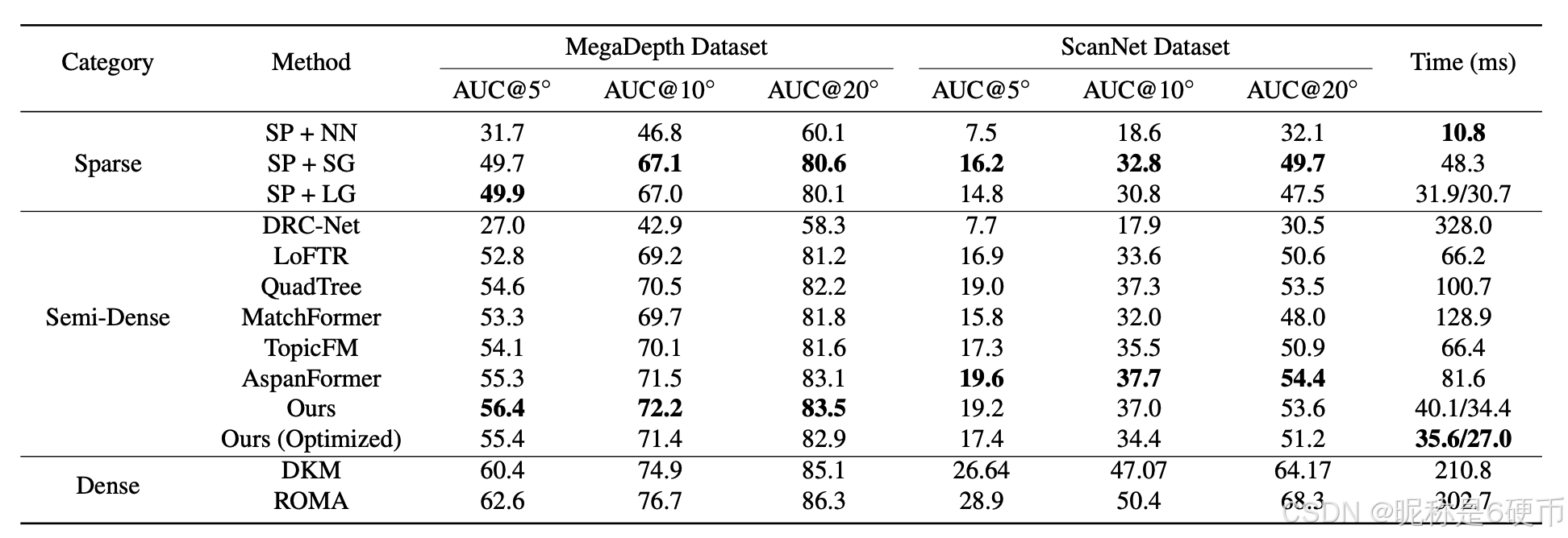
Table 1. Results of Relative Pose Estimation on MegaDepth Dataset and ScanNet Dataset. We use the models trained on the MegaDepth dataset to evaluate all methods on both datasets, which can show the intra- and inter-dataset generalization abilities. The AUC of pose error at different thresholds, along with the processing time for matching image pair at a resolution of 640 × 480 640\times480 640×480 , is presented. For S P + L G \mathrm{SP}+\mathrm{LG} SP+LG , Ours, and Ours (Optimized), the running times of the model using FP32/Mixed-Precision numerical precisions are shown.
【翻译】表1. MegaDepth数据集和ScanNet数据集上的相对位姿估计结果。我们使用在MegaDepth数据集上训练的模型在两个数据集上评估所有方法,这可以展示数据集内和跨数据集的泛化能力。报告了不同阈值下位姿误差的AUC,以及在 640 × 480 640\times480 640×480分辨率下匹配图像对的处理时间。对于 S P + L G \mathrm{SP}+\mathrm{LG} SP+LG、Ours和Ours (Optimized),显示了使用FP32/混合精度数值精度的模型运行时间。
4. Experiments
In this section, we evaluate the performance of our method on several downstream tasks, including homography estimation, pairwise pose estimation and visual localization. Furthermore, we evaluate the effectiveness of our design by conducting detailed ablation studies.
We adopt RepVGG 11 as our feature backbone, and selfand cross-attention are interleaved for N = 4 N=4 N=4 times to transform coarse features. For each attention, we aggregate features by a depth-wise convolution layer and a max-pooling layer, both with a kernel size of 4 × 4 4\times4 4×4 . Our model is trained on the MegaDepth dataset 28, which is a large-scale outdoor dataset. The test scenes are separated from training data following 50. The loss function's weights α \alpha α and β \beta β are set to 1.0 and 0.25, respectively. We use the AdamW optimizer with an initial learning rate of 4 × 10 − 3 4\times10^{-3} 4×10⁻³ . The network training takes about 15 hours with a batch size of 16 on 8 NVIDIA V100 GPUs. And the coarse and fine stages are trained together from scratch. The trained model on MegaDepth is used to evaluate all datasets and tasks in our experiments to demonstrate the generalization ability.
Datasets. We use the outdoor MegaDepth 28 dataset and indoor ScanNet 8 dataset for the evaluation of relative pose estimation to demonstrate the efficacy of our method.
MegaDepth dataset is a large-scale dataset containing sparse 3D reconstructions from 196 scenes. The key challenges on this dataset are large viewpoints and illumination changes, as well as repetitive patterns. We follow the test split of the previous method 50 that uses 1500 sampled pairs from scenes "Sacre Coeur" and "St. Peter's Square" for evaluation. Images are resized so that the longest edge equals 1200 for all semi-dense and dense methods. Following 30, sparse methods are provided resized images with longest edge equals 1600.
ScanNet dataset contains 1613 sequences with groundtruth depth maps and camera poses. They depict indoor scenes with viewpoint changes and texture-less regions. We use the sampled test pairs from 43 for the evaluation, where images are resized to 640 × 480 640\times480 640×480 for all methods.
Baselines. We compare the proposed method with three categories of methods: 1) sparse keypoint detection and matching methods, including SuperPoint 10 with NearestNeighbor (NN), SuperGlue (SG) 43, LightGlue (LG) 30 matchers, 2) semi-dense matchers, including DRC-Net 27, LoFTR 50, QuadTree Attention 52, MatchFormer 59, AspanFormer 7, TopicFM 18, and 3) state-of-the-art dense matcher ROMA 15 that predict matches for each pixel.
Evaluation protocol. Following previous methods, the recovered relative poses by matches are evaluated for reflecting matching accuracy. The pose error is defined as the maximum of angular errors in rotation and translation. We report the AUC of the pose error at thresholds ( 5 ∘ , 10 ∘ (5^{\circ},10^{\circ} (5∘,10∘ , and 20 ∘ 20^{\circ} 20∘ ). Moreover, the running time of matching each image pair in the ScanNet dataset is reported for comprehensively understanding the matching accuracy and efficiency balance. We use a single NVIDIA 3090 to evaluate the running time of all methods.
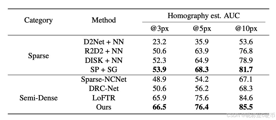
Table 2. Results of Homography Estimation on HPatches Dataset. Our method is compared with sparse and semi-dense methods. The AUC of reprojection error of corner points at different thresholds is reported.
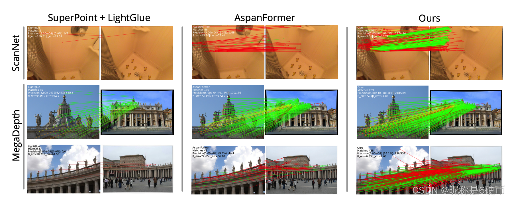
Results. As shown in Tab. 1, the proposed method achieves competitive performances compared with sparse and semidense methods on both datasets. Qualitative comparisons are shown in Fig. 4. Specifically, our method outperforms the best semi-dense baseline AspanFormer on all metrics of the MegaDepth dataset and has lower but comparable performance on the ScanNet dataset, with ∼ 2 \sim2 ∼2 times faster. Our optimized model that eliminates the dual-softmax operator in coarse-level matching further brings efficiency improvements, with slight performance decreases. Using this strategy, our method can outperform the efficient and robust sparse method S P + L G \mathrm{SP}+\mathrm{LG} SP+LG in efficiency with significantly higher accuracy. Dense matcher ROMA shows remarkable matching capability but is slow for applications in practice. Moreover, since ROMA utilizes the pre-trained DINOv2 37 backbone, its strong generalizability on ScanNet may be attributed to the similar indoor training data in DINOv2, where other methods are trained on outdoor MegaDepth only. Compared with it, our method is ∼ 7.5 \sim7.5 ∼7.5 times faster, which has a good balance between accuracy and efficiency.
【翻译】结果。如表1所示,所提出的方法在两个数据集上与稀疏和半密集方法相比都取得了有竞争力的性能。定性比较如图4所示。具体而言,我们的方法在MegaDepth数据集的所有指标上都优于最佳半密集基线AspanFormer,在ScanNet数据集上性能略低但相当,速度快约2倍。我们的优化模型消除了粗粒度匹配中的双softmax算子,进一步提高了效率,性能略有下降。使用这种策略,我们的方法在效率上可以超越高效且鲁棒的稀疏方法 S P + L G \mathrm{SP}+\mathrm{LG} SP+LG,同时具有显著更高的精度。密集匹配器ROMA显示出卓越的匹配能力,但在实际应用中速度较慢。此外,由于ROMA使用预训练的DINOv2 37骨干网络,其在ScanNet上的强泛化能力可能归因于DINOv2中类似的室内训练数据,而其他方法仅在户外MegaDepth上训练。与之相比,我们的方法快约7.5倍,在精度和效率之间取得了良好的平衡。
4.3. 单应性估计
Dataset. We evaluate our method on HPatches dataset 3. HPatches dataset depicts planar scenes divided into sequences. Images are taken under different viewpoints or illumination changes.
Baselines. We compare our method with sparse methods including D2Net 12, R2D2 38, DISK 57 detectors with NN matcher, and SuperPoint10 + SuperGlue 43. As for semi-dense methods, we compare with Sparse-NCNet 40, DRC-Net 27, and LoFTR 50. For SuperGlue and all semidense methods, we use their models trained on MegaDepth dataset for evaluation.
Evaluation Protocol. Following SuperGlue 43 and LoFTR 50, we resize all images for matching so that their smallest edge equals 480 pixels. We collect the mean reprojection error of corner points, and report the area under the cumulative curve (AUC) under 3 different thresholds, including 3 px, 5 px, and 10 px . For all baselines, we employ the same RANSAC method as a robust homography estimator for a fair comparison. Following LoFTR, we select only the top 1000 predicted matches of semi-dense methods for the sake of fairness.
Results. As shown in Tab. 2, even though the number of matches is restricted, our method can also work remarkably well and outperform sparse methods significantly. Compared with semi-dense, our method can surpass them with significantly higher efficiency. We attribute this to the effectiveness of two-stage refinement for accuracy improvement and proposed aggregation module for efficiency.
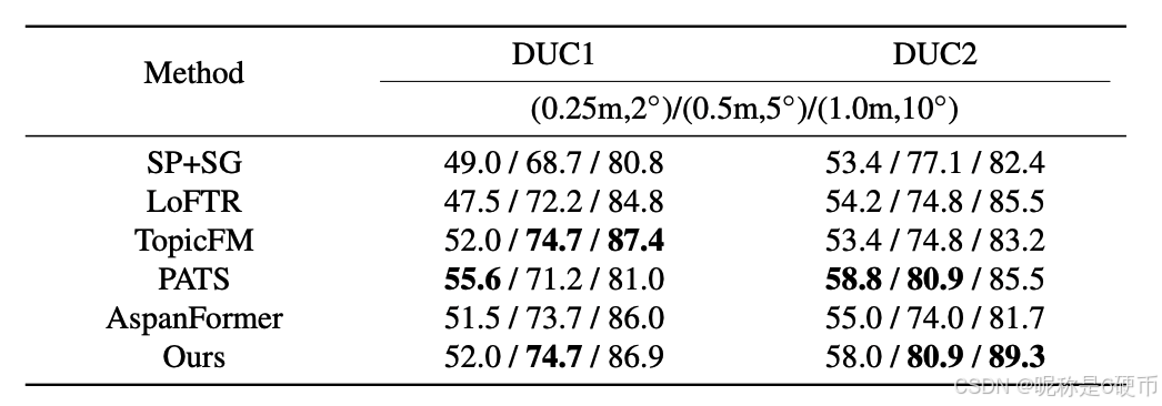
Table 3. Results of Visual Localization on InLoc Dataset.
【翻译】表3. InLoc数据集上的视觉定位结果。
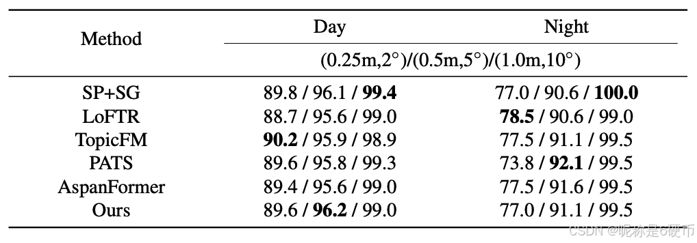
Table 4. Results of Visual Localization on Aachen v1.1 Dataset.
【翻译】表4. Aachen v1.1数据集上的视觉定位结果。
4.4. 视觉定位
Datasets and Evaluation Protocols. Visual localization is an important downstream task of image matching, which aims to estimate the 6-DoF poses of query images based on the 3D scene model. We conduct experiments on two commonly used benchmarks, including InLoc 51 dataset and Aachen v1.1 45 dataset, for evaluation to demonstrate the superiority of our method. InLoc dataset is captured on indoor scenes with plenty of repetitive structures and textureless regions, where each database image has a corresponding depth map. Aachen v1.1 is a challenging large-scale outdoor dataset for localization with large-viewpoint and day-andnight illumination changes, which particularly relies on the robustness of matching methods. We adopt its full localization track for benchmarking.
Following 7, 50, the open-sourced localization framework HLoc 42 is utilized. For both datasets, the percentage of pose errors satisfying both angular and distance thresholds is reported following the benchmarks, where different thresholds are used. For the InLoc dataset, the metrics of two test scenes including DUC1 and DUC2 are separately reported. As for the Aachen v1.1 dataset, the metrics corresponding to the daytime and nighttime divisions are reported.
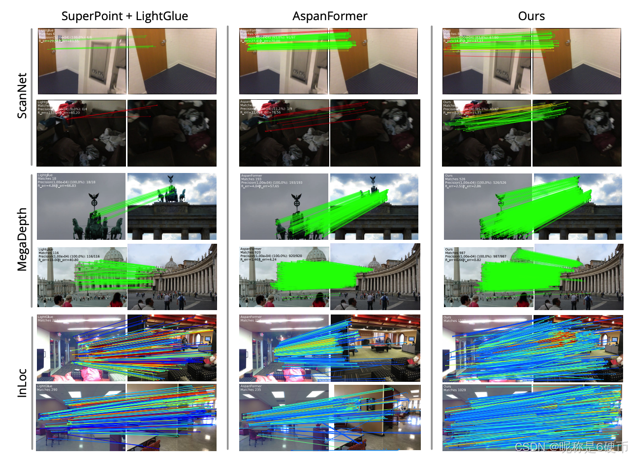
Figure 4. Qualitative Results. Our method is compared with the sparse matching pipeline SuperPoint 10+LightGlue 30, semi-dense matcher AspanFormer 7. Image pairs with texture-poor regions and large-viewpoint changes can be robustly matched by our method. The red color indicates epipolar error beyond 5 × 10 − 4 5\times10^{-4} 5×10⁻⁴ (in the normalized image coordinates).
Baselines. We compare the proposed method with both detector-based method SuperPoint10 + SuperGlue 43 and detector-free methods including LoFTR 50, TopicFM 18, PATS 36 and Aspanformer 7.
Results. We adhere to the pipeline and evaluation settings of the online visual localization benchmark(https://www.visuallocalization.net/benchmark) to ensure fairness. As presented in Tab. 3, the proposed method achieves competitive results, taking both detector-based and detectorfree methods into account. Being a method primarily geared towards efficiency, our approach can deliver results comparable to those of many accuracy-oriented methods. As depicted in Tab. 4, our method also demonstrates performance on par with the best-performing approaches.
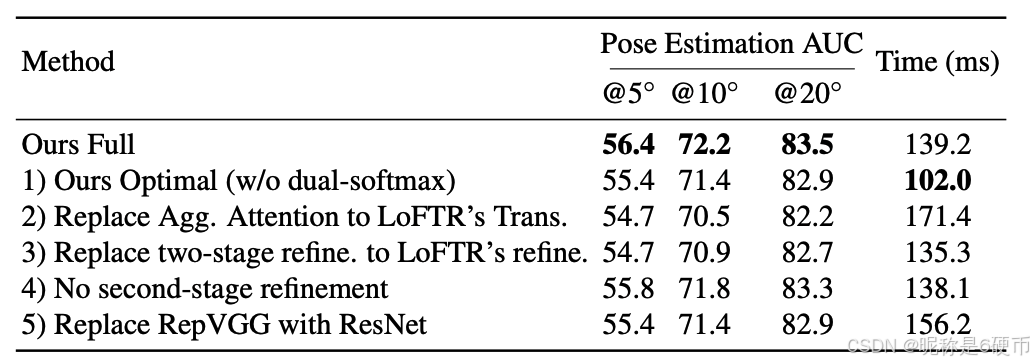
Table 5. Ablation Studies. The components of our method are ablated on the MegaDepth dataset for a comprehensive understanding of our method, where averaged running times for an image pair with high-resolution 1200 × 1200 1200\times1200 1200×1200 are reported.
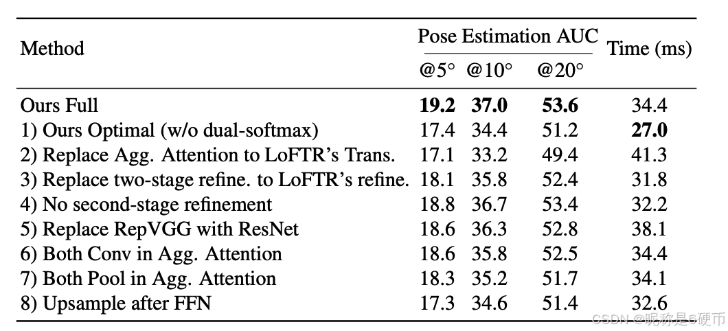
In this part, we conduct detailed ablation studies to analyze the effectiveness of our proposed modules with results shown in Tab. 5. 1) Without dual-softmax, our optimal model can bring huge efficiency improvement in high-resolution images. 2) In coarse feature transformation, replacing the proposed aggregated attention module with LoFTR's transformer can bring significant efficiency dropping, as well as accuracy decrease. Note that the replaced transformer is also equipped with RoPE same as ours for fair comparison. This demonstrates the efficacy of the proposed module that performing vanilla attention on aggregated features can achieve higher efficiency with even better matching accuracy. 3) Compared with using LoFTR's refinement that performs expectation on the entire correlation patch, the proposed two-stage refinement layer can bring accuracy improvement with neglectable latency. We attribute this to the two-stage refinement's property that can maximize the suppression of location variance in correlation refinement. 4) Dropping the second refinement stage will lead to degraded pose accuracy with minor efficiency changes, especially on the strict A U C @ 5 ∘ \operatorname{AUC@5^{\circ}} AUC@5∘ metric. 5) Changing the backbone from reparameterized VGG 11 back to multi-branch ResNet 20 leads to decreased efficiency with similar accuracy, which demonstrates the effectiveness of our design choice for efficiency.
This paper introduces a new semi-dense local feature matcher based on the success of LoFTR. We revisit its designs and propose several improvements for both efficiency and matching accuracy. A key observation is that performing the Transformer on the entire coarse feature map is redundant due to the similar local information, where an aggregated attention module is proposed to perform transformer on reduced tokens with significantly better efficiency and competitive performance. Moreover, a two-stage correlation layer is devised to solve the location variance problem in LoFTR's refinement design, which further brings accuracy improvements. As a result, our method can achieve ∼ 2.5 \sim2.5 ∼2.5 times faster compared with LoFTR with better matching accuracy. Moreover, as a semi-dense matching method, the proposed method can achieve comparable efficiency with the recent robust sparse feature matcher LightGlue 30. We believe this opens up the applications of our method in large-scale or latency-sensitive downstream tasks, such as image retrieval and 3D reconstruction. Please refer to the supplementary material for discussions about limitations and future works.
Some previous works explored using pooling in ViT but are with different design choices from our method due to different tasks. PoolFormer 61 replaces the multi-head attention with pooling, which cannot be used for cross-attention in matching that two images are not pixel-aligned. MVit 16 uses pooling to reduce tokens like ours, but they cannot get high-res features that are required for matching.
【翻译】一些先前的工作探索了在 ViT 中使用池化,但由于任务不同,它们的设计选择与我们的方法不同。PoolFormer 61 用池化替换了多头注意力,这不能用于匹配中的交叉注意力,因为两幅图像不是像素对齐的。MVit 16 像我们一样使用池化来减少 token,但它们无法获得匹配所需的高分辨率特征。
Differently, we propose to first conduct attention on aggregated features and then upsample before feed-forward network (FFN) for later fusion with input feature, as shown in Fig. 3. This aggregate-and-upsample block can minimize information loss in aggregation and efficiently get high-res informative features, where conducting upsampling before fusion is crucial to fuse smoothly interpolated messages with a detailed feature map. Ablation is in Tab. 10 (8).
Moreover, We perform Conv on Q value instead of pooling because salient tokens should not represent neighbors to query attention. The transformer is crucial for enhancing non-salient features for matching. Pooling on Q causes the attention of texture-less areas dominated by neighboring salient tokens, reducing the performance as ablated in Tab. 10 (6,7).
RepVGG 11 blocks are used to build a four-stage feature backbone. We use a width of 64 and a stride of 1 for the first stage and widths of 64, 128, 256 and strides of 2 for the subsequent three stages. Each stage is composed of 1, 2, 4, 14 RepVGG blocks and ReLU activations, respectively. The output of the last stage in 1 / 8 1/8 1/8 image resolution is used for efficient local feature transformer modules to get attended coarse feature maps. The second and third stages' feature maps are in 1 / 2 1/2 1/2 and 1 / 4 1/4 1/4 image resolutions, respectively, which are used for fusing with transformed coarse features for fine features.
We use the 2D extension of Rotary position encoding 49 to encode the relative position between coarse features in selfattention modules. Given the projected features q q q and k k k , the attention score between two features q i q_{i} qi and k j k_{j} kj is computed as:
【翻译】我们使用旋转位置编码 49 的 2D 扩展来编码自注意力模块中粗糙特征之间的相对位置。给定投影特征 q q q 和 k k k,两个特征 q i q_{i} qi 和 k j k_{j} kj 之间的注意力分数计算如下:
a i j = q i T R ( x j − x i , y j − y i ) k j , a_{i j}=q_{i}^{T}R(x_{j}-x_{i},y_{j}-y_{i})k_{j}\mathrm{~,~} aij=qiTR(xj−xi,yj−yi)kj ,
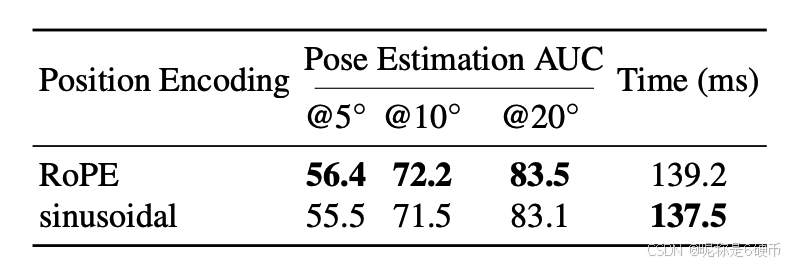
Table 6. Impact of position encoding on the MegaDepth dataset, where averaged running times for an image pair with highresolution 1200 × 1200 1200\times1200 1200×1200 are reported.
where x i , y i , x j , y j x_{i},y_{i},x_{j},y_{j} xi,yi,xj,yj are the coordinates of q i q_{i} qi and k j k_{j} kj , R R R is a block diagonal matrix:
【翻译】其中 x i , y i , x j , y j x_{i},y_{i},x_{j},y_{j} xi,yi,xj,yj 是 q i q_{i} qi 和 k j k_{j} kj 的坐标, R R R 是一个分块对角矩阵:
R ( Δ x , Δ y ) = ( R 1 ( Δ x , Δ y ) R 2 ( Δ x , Δ y ) ⋱ R d / 4 ( Δ x , Δ y ) ) R(\Delta x,\Delta y) = \begin{pmatrix} R_1(\Delta x,\Delta y) & & & \\ & R_2(\Delta x,\Delta y) & & \\ & & \ddots & \\ & & & R_{d/4}(\Delta x,\Delta y) \end{pmatrix} R(Δx,Δy)= R1(Δx,Δy)R2(Δx,Δy)⋱Rd/4(Δx,Δy)
R k ( Δ x , Δ y ) = ( cos ( θ k Δ x ) − sin ( θ k Δ x ) 0 0 sin ( θ k Δ x ) cos ( θ k Δ x ) 0 0 0 0 cos ( θ k Δ y ) − sin ( θ k Δ y ) 0 0 sin ( θ k Δ y ) cos ( θ k Δ y ) ) R_k(\Delta x,\Delta y) = \begin{pmatrix} \cos(\theta_k \Delta x) & -\sin(\theta_k \Delta x) & 0 & 0 \\ \sin(\theta_k \Delta x) & \cos(\theta_k \Delta x) & 0 & 0 \\ 0 & 0 & \cos(\theta_k \Delta y) & -\sin(\theta_k \Delta y) \\ 0 & 0 & \sin(\theta_k \Delta y) & \cos(\theta_k \Delta y) \end{pmatrix} Rk(Δx,Δy)= cos(θkΔx)sin(θkΔx)00−sin(θkΔx)cos(θkΔx)0000cos(θkΔy)sin(θkΔy)00−sin(θkΔy)cos(θkΔy)
where θ k = 1 10000 4 k / d , k ∈ 1 , 2 , . . . , d / 4 \begin{array}{r}{\theta_{k}=\frac{1}{10000^{4k/d}},k\in1,2,...,d/4}\end{array} θk=100004k/d1,k∈1,2,...,d/4 encode the index of feature channels.
【翻译】其中 θ k = 1 10000 4 k / d , k ∈ 1 , 2 , . . . , d / 4 \begin{array}{r}{\theta_{k}=\frac{1}{10000^{4k/d}},k\in1,2,...,d/4}\end{array} θk=100004k/d1,k∈1,2,...,d/4 编码特征通道的索引。
Compared to the absolute position encoding used in previous methods 7, 18, 36, 50, 52, 59, we utilize 2D RoPE to allow the model to focus more on the interaction between features rather than their specific locations, which benefits capturing the context of local features. Moreover, relative position encoding is more robust to transformations like rotation, translation, and scaling, which is important for matching local features in different views.
Position Encoding We compare the performance of our 2D RoPE with the sinusoidal position encoding 58 in Tab. 6. The results show that using 2D RoPE can achieve better performance than sinusoidal position encoding.
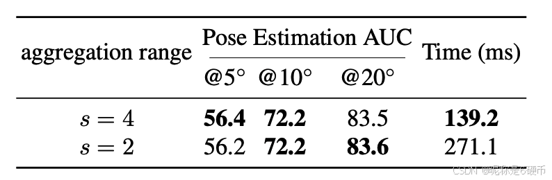
Aggregation Range We show the performance of our method with different aggregation range s s s in Tab. 7. In our aggregated attention module, we use a 4 × 4 4\times4 4×4 aggregation range to reduce token size before performing attention. Using a smaller aggregation range leads to more tokens, with slight performance changes but significantly slower matching speed. This validates the effectiveness of our parameter choice in the aggregation attention module.
【翻译】聚合范围 我们在表 7 中展示了我们的方法在不同聚合范围 s s s 下的性能。在我们的聚合注意力模块中,我们使用 4 × 4 4\times4 4×4 的聚合范围在执行注意力之前减少 token 大小。使用较小的聚合范围会导致更多的 token,性能变化轻微但匹配速度显著变慢。这验证了我们在聚合注意力模块中参数选择的有效性。
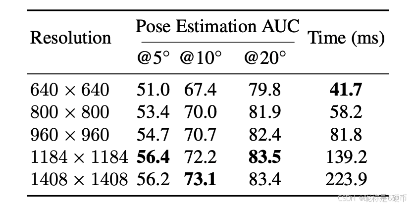
Image Resolution We test the performance of our method with different image resolutions to show the performance and efficiency changes. Results are shown in Tab. 8. Compared with the default resolution 1184 × 1184 1184\times1184 1184×1184 used in the MegaDepth evaluation, using a larger image size leads to noticeable accuracy improvement with a slower matching speed. Our method can still achieve competitive performance using low-resolution 640 × 640 640\times640 640×640 images with the fastest speed. Therefore, our method is pretty robust in image resolution choices for flexible real-world applications.
Figure 5. Qualitative Results. Our method is compared with the sparse matching pipeline SuperPoint 10+LightGlue 30, semi-dense matcher AspanFormer 7. The red color indicates epipolar error beyond 5 × 10 − 4 5\times10^{-4} 5×10⁻⁴ on ScanNet and 1 × 10 − 4 1\times10^{-4} 1×10⁻⁴ on MegaDepth (in the normalized image coordinates). Since no ground-truth pose is available on InLoc dataset, we color the match with predicted confidence. Red indicates higher confidence and blue for the opposite.
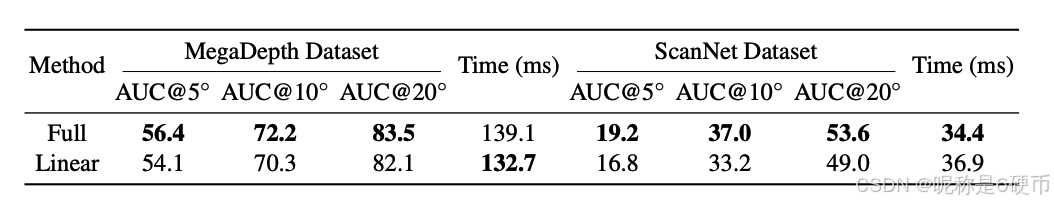
Linear Attention After Aggregation Using linear attention in our aggregated attention module introduces minor efficiency gain on high-resolution but with accuracy dropping as shown in Tab. 9.
Additional ablation studies on the ScanNet dataset We further repeat the ablation studies in the main paper and conduct additional ablation studies on the ScanNet dataset to validate the design choices of our proposed modules. Results are shown in Tab. 10.
Table 7. Impact of aggregation range on the MegaDepth dataset, where averaged running times for an image pair with highresolution 1200 × 1200 1200\times1200 1200×1200 are reported.
Table 8. Impact of test image resolution on the MegaDepth dataset.
【翻译】表 8. 测试图像分辨率对 MegaDepth 数据集的影响。
Table 9. Impact of linear attention after aggregation on the MegaDepth and ScanNet dataset, where the resolution are 1200 × 1200 1200\times 1200 1200×1200 and 640 × 480 640\times480 640×480 , respectively.
Table 10. The components of our method are ablated on the ScanNet dataset again for a comprehensive understanding of our method, where averaged running times for an image pair with resolution 640 × 480 640\times480 640×480 are reported.
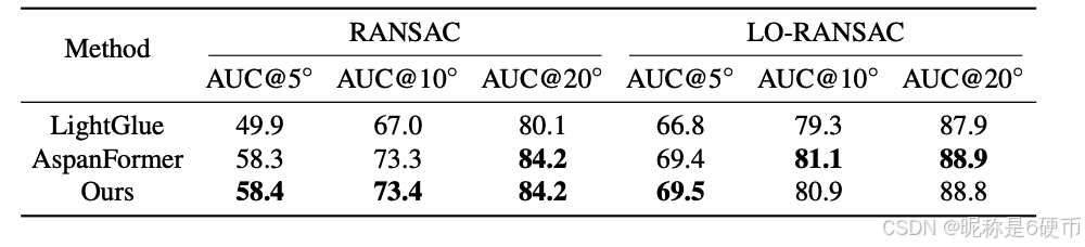
LightGlue uses a RANSAC setting different from other baseline papers 7, 14, 15, 18, 43, 50, 52, 59 in relative pose estimation evaluations on MegaDepth. We further conduct experiments following LightGlue's setting (OpenCV RANSAC 17 and LO-RANSAC 25 with carefully tuned RANSAC inlier thresholds), as shown in Tab. 11. Using the naive RANSAC method, the performance gap between ours and LightGlue becomes larger after RANSAC threshold tuning (compared with our untuned results in Tab. 1). This demonstrates that our method can achieve significantly better accuracy without depending on the sophisticated modern RANSAC method, thereby revealing its superior match quality. Using the stronger outlier filter LO-RANSAC, the accuracy of all methods is boosted and our method consistently achieves better performance than LightGlue, especially on the A U C 5 ∘ \mathrm{AUC5^{\circ}} AUC5∘ metric.
Table 11. Results of Relative Pose Estimation on MegaDepth Dataset following LightGlue's setting. The AUC of pose error at different thresholds is presented.
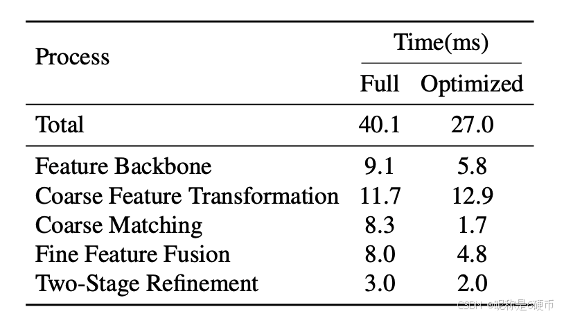
Table 12. Time cost for an image pair of 640 × 480 640\times480 640×480 on the ScanNet dataset. The optimized model uses Mixed-Precision numerical accuracy and drops the dual-softmax operator in the coarse matching phase.
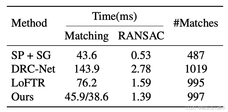
Table 13. Running times of different methods on HPatches dataset. All images are resized so that their short edge equals 480 pixels following SuperGlue 43 and LoFTR 50. For Ours, the running times of the model using FP32/Mixed-Precision numerical precisions are shown.
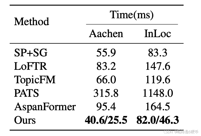
Table 14. Running times of different methods on Aachen and InLoc dataset. To measure the running time, we sample 818 and 356 pairs of images from the NetVLAD 2's retrieval results for Aachen and InLoc, respectively. All images are resized so that their long edge equals 1024 pixels following HLoc 42. For Ours, the running times of the model using FP32/Mixed-Precision numerical precisions are shown.
The running times evaluated in the paper are averaged over all pairs in the test dataset with a warm-up of 50 pairs for accurate measurement. All the methods are tested on a single NVIDIA RTX 3090 GPU with 14 cores of Intel Xeon Gold 6330 CPU.
We further report each part running time of our method in Tab. 12, where both full and optimized models are shown. We noticed that skipping the dual-softmax of Coarse Matching in the optimized model can significantly reduce the running time. What's more, with the benefit of Mixed-Precision, the running time of feature extraction can be further reduced.
The latency on 3 datasets included in Tabs. 2 to 4 are shown in Tab. 13 and Tab. 14, where conclusion and speed rankings are the same as indicated in Tab. 1. We further show RANSAC time on HPatches dataset. Both matching and RANSAC latency of our method are smaller than LoFTR with a similar number of matches.
We find that our method may fail when strong repetitive structures exist, such as matching an image pair that depicts different scenes containing the same chair. We think this may be due to the current model focusing more on local features for accurate matching, where global semantic context is lacking. Therefore, the mechanism of high-level contexts can be added to the model for performance improvement on ambiguous scenes. Moreover, we believe the efficiency of our method can be further improved by adopting the early stop strategy of LightGlue 30 since the contribution of the proposed efficient aggregation module is orthogonal to it.