We present a novel method for local image feature matching. Instead of performing image feature detection, description, and matching sequentially, we propose to first establish pixel-wise dense matches at a coarse level and later refine the good matches at a fine level. In contrast to dense methods that use a cost volume to search correspondences, we use self and cross attention layers in Transformer to obtain feature descriptors that are conditioned on both images. The global receptive field provided by Transformer enables our method to produce dense matches in low-texture areas, where feature detectors usually struggle to produce repeatable interest points. The experiments on indoor and outdoor datasets show that LoFTR outperforms state-of-the-art methods by a large margin. LoFTR also ranks first on two public benchmarks of visual localization among the published methods. Code is available at our project page: https://zju3dv.github.io/loftr/.
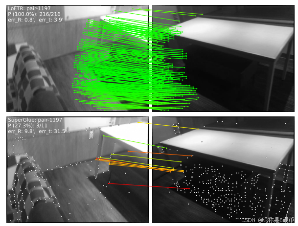
Figure 1: Comparison between the proposed method LoFTR and the detector-based method SuperGlue 37. This example demonstrates that LoFTR is capable of finding correspondences on the texture-less wall and the floor with repetitive patterns, where detector-based methods struggle to find repeatable interest points. (Only the inlier matches after RANSAC are shown. The green color indicates a match with epipolar error smaller than 5 × 10 − 4 5 \times 10^{-4} 5×10⁻⁴ (in the normalized image coordinates).)
Local feature matching between images is the cornerstone of many 3D computer vision tasks, including structure from motion (SfM), simultaneous localization and mapping (SLAM), visual localization, etc. Given two images to be matched, most existing matching methods consist of three separate phases: feature detection, feature description, and feature matching. In the detection phase, salient points like corners are first detected as interest points from each image. Local descriptors are then extracted around neighborhood regions of these interest points. The feature detection and description phases produce two sets of interest points with descriptors, the point-to-point correspondences of which are later found by nearest neighbor search or more sophisticated matching algorithms.
The use of a feature detector reduces the search space of matching, and the resulted sparse correspondences are sufficient for most tasks, e.g., camera pose estimation. However, a feature detector may fail to extract enough interest points that are repeatable between images due to various factors such as poor texture, repetitive patterns, viewpoint change, illumination variation, and motion blur. This issue is especially prominent in indoor environments, where low-texture regions or repetitive patterns sometimes occupy most areas in the field of view. Fig. 1 shows an example. Without repeatable interest points, it is impossible to find correct correspondences even with perfect descriptors.
Several recent works 34, 33, 19 have attempted to remedy this problem by establishing pixel-wise dense matches. Matches with high confidence scores can be selected from the dense matches, and thus feature detection is avoided. However, the dense features extracted by convolutional neural networks (CNNs) in these works have limited receptive field which may not distinguish indistinctive regions. Instead, humans find correspondences in these indistinctive regions not only based on the local neighborhood, but with a larger global context. For example, low-texture regions in Fig. 1 can be distinguished according to their relative positions to the edges. This observation tells us that a large receptive field in the feature extraction network is crucial.
Motivated by the above observations, we propose Local Feature TRansformer (LoFTR), a novel detector-free approach to local feature matching. Inspired by seminal work SuperGlue 37, we use Transformer 48 with self and cross attention layers to process (transform) the dense local features extracted from the convolutional backbone. Dense matches are first extracted between the two sets of transformed features at a low feature resolution ( 1 / 8 (1/8 (1/8 of the image dimension). Matches with high confidence are selected from these dense matches and later refined to a subpixel level with a correlation-based approach. The global receptive field and positional encoding of Transformer enable the transformed feature representations to be contextand position-dependent. By interleaving the self and cross attention layers multiple times, LoFTR learns the denselyarranged globally-consented matching priors exhibited in the ground-truth matches. A linear transformer is also adopted to reduce the computational complexity to a manageable level.
We evaluate the proposed method on several image matching and camera pose estimation tasks with indoor and outdoor datasets. The experiments show that LoFTR outperforms detector-based and detector-free feature matching baselines by a large margin. LoFTR also achieves stateof-the-art performance and ranks first among the published methods on two public benchmarks of visual localization. Compared to detector-based baseline methods, LoFTR can produce high-quality matches even in indistinctive regions with low-textures, motion blur, or repetitive patterns.
Detector-based Local Feature Matching. Detector-based methods have been the dominant approach for local feature matching. Before the age of deep learning, many renowned works in the traditional hand-crafted local features have achieved good performances. SIFT 26 and ORB 35 are arguably the most successful hand-crafted local features and are widely adopted in many 3D computer vision tasks. The performance on large viewpoint and illumination changes of local features can be significantly improved with learning-based methods. Notably, LIFT 51 and MagicPoint 8 are among the first successful learning-based local features. They adopt the detectorbased design in hand-crafted methods and achieve good performance. SuperPoint 9 builds upon MagicPoint and proposes a self-supervised training method through homographic adaptation. Many learning-based local features along this line 32, 11, 25, 28, 47 also adopt the detectorbased design.
The above-mentioned local features use the nearest neighbor search to find matches between the extracted interest points. Recently, SuperGlue 37 proposes a learningbased approach for local feature matching. SuperGlue accepts two sets of interest points with their descriptors as input and learns the matching through a graph neural network with attention. However, SuperGlue still relies on a feature detector to extract interest points, and thus suffers from the same repeatability issue. In contrast, LoFTR is a detector-free method that establishes matches at the pixel level.
Transformers in Vision Related Tasks. Transformer 48 has become the de facto standard for sequence modeling in natural language processing (NLP) due to their simplicity and computation efficiency. Recently, Transformers are also getting more attention in computer vision tasks, such as image classification 10, object detection 3, and video understanding 1, 2. The self-attention mechanism in Transformers provides a global receptive field, which is beneficial for capturing long-range dependencies. In this work, we leverage the global receptive field of Transformers to extract context-dependent features for local feature matching.
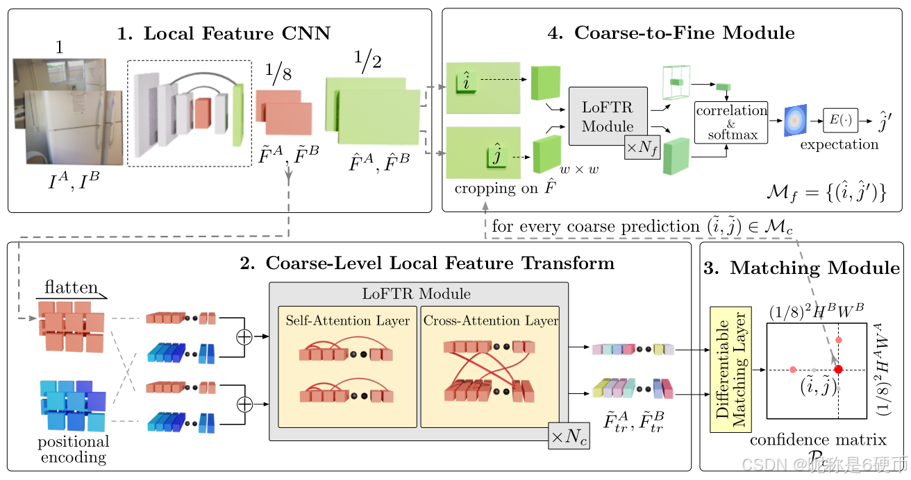
Figure 2: Overview of the proposed method. LoFTR has four components: 1. A local feature CNN extracts the coarse-level feature maps F ~ A \tilde{F}^{A} F~A and F ~ B \tilde{F}^{B} F~B , together with the fine-level feature maps F ^ A {\hat{F}}^{A} F^A and F ^ B {\hat{F}}^{B} F^B from the image pair I A I^{A} IA and I B I^{B} IB (Section 3.1). 2. The coarse feature maps are flattened to 1-D vectors and added with the positional encoding. The added features are then processed by the Local Feature TRansformer (LoFTR) module, which has N c N_{c} Nc self-attention and cross-attention layers (Section 3.2). 3. A differentiable matching layer is used to match the transformed features, which ends up with a confidence matrix P c \mathcal{P}{c} Pc . The matches in P c \mathcal{P}{c} Pc are selected according to the confidence threshold and mutual-nearest-neighbor criteria, yielding the coarse-level match prediction M c \mathcal{M}{c} Mc (Section 3.3). 4. For every selected coarse prediction ( i ~ , j ~ ) ∈ M c (\tilde{i},\tilde{j})\in{\mathcal{M}}{c} (i~,j~)∈Mc , a local window with size w × w w\times w w×w is cropped from the fine-level feature map. Coarse matches will be refined within this local window to a sub-pixel level as the final match prediction M f \mathcal{M}_{f} Mf (Section 3.4).
【翻译】图2:所提出方法的概述。LoFTR有四个组件:1. 局部特征CNN从图像对 I A I^{A} IA和 I B I^{B} IB中提取粗级别特征图 F ~ A \tilde{F}^{A} F~A和 F ~ B \tilde{F}^{B} F~B,以及细级别特征图 F ^ A {\hat{F}}^{A} F^A和 F ^ B {\hat{F}}^{B} F^B(第3.1节)。2. 粗特征图被展平为1维向量并添加位置编码。添加后的特征随后由局部特征变换器(LoFTR)模块处理,该模块具有 N c N_{c} Nc个自注意力和交叉注意力层(第3.2节)。3. 使用可微分匹配层来匹配转换后的特征,最终得到置信度矩阵 P c \mathcal{P}{c} Pc。根据置信度阈值和互最近邻准则从 P c \mathcal{P}{c} Pc中选择匹配,产生粗级别匹配预测 M c \mathcal{M}{c} Mc(第3.3节)。4. 对于每个选定的粗预测 ( i ~ , j ~ ) ∈ M c (\tilde{i},\tilde{j})\in{\mathcal{M}}{c} (i~,j~)∈Mc,从细级别特征图中裁剪出大小为 w × w w\times w w×w的局部窗口。粗匹配将在此局部窗口内被细化到亚像素级别,作为最终匹配预测 M f \mathcal{M}_{f} Mf(第3.4节)。
【解析】LoFTR采用粗到精的分层匹配策略,通过四个组件完成从图像对到精确匹配的转换。第一个组件是特征提取阶段,使用CNN同时生成两个不同分辨率层次的特征表示。粗级别特征图 F ~ A \tilde{F}^{A} F~A和 F ~ B \tilde{F}^{B} F~B通常是原图尺寸的 1 / 8 1/8 1/8,这个较低的分辨率能够显著减少后续Transformer处理的计算量,同时保留足够的语义信息用于建立对应关系。细级别特征图 F ^ A {\hat{F}}^{A} F^A和 F ^ B {\hat{F}}^{B} F^B则保持更高的空间分辨率,例如原图的 1 / 2 1/2 1/2或 1 / 4 1/4 1/4,这些特征包含更丰富的空间细节,为后续的精细化匹配提供必要的高频信息。第二个组件处理粗级别特征,首先将二维特征图展平成一维序列,这是为了适配Transformer的输入格式要求。展平操作将空间维度 ( H , W ) (H,W) (H,W)转换为序列长度 N = H × W N=H\times W N=H×W。接着为每个位置添加位置编码,这个步骤至关重要,因为Transformer本身对输入序列的顺序是不敏感的,位置编码通过正弦和余弦函数的组合为每个空间位置赋予唯一的位置标识,使得网络能够区分空间上不同位置的特征,即使这些位置的外观特征相似。经过位置编码增强的特征随后进入LoFTR模块,这个模块由 N c N_{c} Nc层自注意力和交叉注意力交替堆叠而成。自注意力层让同一图像内的所有位置特征相互交互,使每个位置能够聚合来自整幅图像的全局上下文信息,这解决了卷积网络感受野有限的问题。交叉注意力层则在两幅图像的特征之间建立联系,让图像 A A A中的每个位置都能感知图像 B B B中所有位置的信息,反之亦然,这为后续的匹配奠定了基础。通过多次交替应用这两种注意力机制,网络能够逐步学习到既考虑单图像内部一致性又考虑跨图像对应关系的特征表示。第三个组件执行粗级别匹配,使用可微分的匹配层计算转换后特征之间的相似度,生成置信度矩阵 P c \mathcal{P}{c} Pc。这个矩阵的每个元素 P c ( i , j ) \mathcal{P}{c}(i,j) Pc(i,j)表示图像 A A A中位置 i i i与图像 B B B中位置 j j j匹配的置信度。为了从这个密集的置信度矩阵中筛选出可靠的匹配,方法采用两个准则:首先设置置信度阈值,只保留置信度超过阈值的候选匹配;然后应用互最近邻准则,即只有当位置 i i i在图像 B B B中的最佳匹配是 j j j,同时位置 j j j在图像 A A A中的最佳匹配也是 i i i时,这对匹配才被接受。这种双向验证机制能够有效过滤掉单向匹配中的许多错误对应。经过筛选后得到的粗级别匹配集合记为 M c \mathcal{M}{c} Mc。第四个组件负责匹配精细化,虽然粗级别匹配已经建立了大致正确的对应关系,但由于粗特征图的分辨率较低,匹配位置的精度有限,通常只能精确到几个像素。为了获得亚像素级别的精确匹配,方法针对每个粗匹配对 ( i ~ , j ~ ) (\tilde{i},\tilde{j}) (i~,j~),在细级别特征图上以粗匹配位置为中心裁剪出大小为 w × w w\times w w×w的局部窗口。在这个局部窗口内进行更精细的搜索,通过计算窗口内所有位置与目标位置的相关性,找到相关性最高的亚像素位置作为精细化后的匹配。这个局部搜索策略既保证了精度,又避免了在整个细特征图上进行全局搜索带来的巨大计算开销。最终输出的匹配集合 M f \mathcal{M}{f} Mf包含了亚像素精度的匹配位置,可以直接用于下游任务如相机位姿估计。整个流程包含从全局到局部、从粗糙到精细的渐进式匹配思想,既利用了Transformer的全局建模能力来处理困难区域的匹配,又通过分层处理控制了计算复杂度,实现了精度和效率的平衡。
3. Methods
Given the image pair I A I^{A} IA and I B I^{B} IB , the existing local feature matching methods use a feature detector to extract interest points. We propose to tackle the repeatability issue of feature detectors with a detector-free design. An overview of the proposed method LoFTR is presented in Fig. 2.
【翻译】给定图像对 I A I^{A} IA和 I B I^{B} IB,现有的局部特征匹配方法使用特征检测器来提取兴趣点。我们提出通过无检测器设计来解决特征检测器的可重复性问题。所提出的LoFTR方法的概述如图2所示。
We use a standard convolutional architecture with FPN 22 (denoted as the local feature CNN) to extract multi-level features from both images. We use F ~ A \tilde{F}^{A} F~A and F ~ B \tilde{F}^{B} F~B to denote the coarse-level features at 1 / 8 1/8 1/8 of the original image dimension, and F ^ A {\hat{F}}^{A} F^A and F ^ B {\hat{F}}^{B} F^B the fine-level features at 1 / 2 1/2 1/2 of the original image dimension.
【翻译】我们使用带有FPN 22的标准卷积架构(称为局部特征CNN)从两幅图像中提取多级特征。我们使用 F ~ A \tilde{F}^{A} F~A和 F ~ B \tilde{F}^{B} F~B表示原始图像尺寸 1 / 8 1/8 1/8处的粗级别特征,使用 F ^ A {\hat{F}}^{A} F^A和 F ^ B {\hat{F}}^{B} F^B表示原始图像尺寸 1 / 2 1/2 1/2处的细级别特征。
Convolutional Neural Networks (CNNs) possess the inductive bias of translation equivariance and locality, which are well suited for local feature extraction. The downsampling introduced by the CNN also reduces the input length of the LoFTR module, which is crucial to ensure a manageable computation cost.
After the local feature extraction, F ~ A \tilde{F}^{A} F~A and F ~ B \tilde{F}^{B} F~B are passed through the LoFTR module to extract position and context dependent local features. Intuitively, the LoFTR module transforms the features into feature representations that are easy to match. We denote the transformed features as F ~ t r A \tilde{F}{t r}^{A} F~trA and F ~ t r B \tilde{F}{t r}^{B} F~trB.
【翻译】在局部特征提取之后, F ~ A \tilde{F}^{A} F~A和 F ~ B \tilde{F}^{B} F~B通过LoFTR模块来提取位置和上下文相关的局部特征。直观地说,LoFTR模块将特征转换为易于匹配的特征表示。我们将转换后的特征表示为 F ~ t r A \tilde{F}{t r}^{A} F~trA和 F ~ t r B \tilde{F}{t r}^{B} F~trB。
【解析】经过CNN提取的粗级别特征 F ~ A \tilde{F}^{A} F~A和 F ~ B \tilde{F}^{B} F~B虽然包含了图像的语义信息,但这些特征是由卷积层独立提取的,每个位置的特征主要依赖于其局部感受野内的信息。这种局部性虽然有助于捕捉纹理和边缘等低层次视觉模式,但在建立跨图像的对应关系时存在局限性。LoFTR模块的核心作用是通过Transformer的自注意力和交叉注意力机制,让特征变得依赖于位置和上下文。位置依赖性通过位置编码实现,使得即使在视觉外观相似的区域,不同空间位置的特征也能被区分开来。上下文依赖性则通过注意力机制实现,每个位置的特征不再是孤立的,而是融合了整幅图像或对应图像中其他位置的信息。转换后的特征 F ~ t r A \tilde{F}{t r}^{A} F~trA和 F ~ t r B \tilde{F}{t r}^{B} F~trB不仅编码了局部外观,还编码了该位置在整体图像结构中的角色以及与另一幅图像中潜在对应位置的关系,这使得后续的匹配过程更加准确和鲁棒。
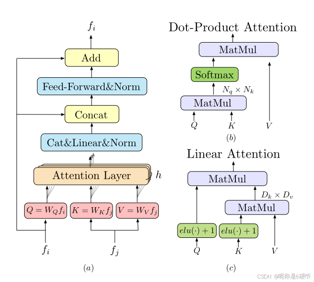
Preliminaries: Transformer 48. We first briefly introduce the Transformer here as background. A Transformer encoder is composed of sequentially connected encoder layers. Fig. 3(a) shows the architecture of an encoder layer.
The key element in the encoder layer is the attention layer. The input vectors for an attention layer are conventionally named query, key, and value. Analogous to information retrieval, the query vector Q Q Q retrieves information from the value vector V V V , according to the attention weight computed from the dot product of Q Q Q and the key vector K K K corresponding to each value V V V . The computation graph of the attention layer is presented in Fig. 3(b). Formally, the attention layer is denoted as:
【翻译】编码器层中的关键元素是注意力层。注意力层的输入向量通常被命名为查询(query)、键(key)和值(value)。类比于信息检索,查询向量 Q Q Q根据从 Q Q Q与每个值 V V V对应的键向量 K K K的点积计算得到的注意力权重,从值向量 V V V中检索信息。注意力层的计算图如图3(b)所示。形式上,注意力层表示为:
【解析】注意力机制的设计灵感来源于人类的选择性注意能力,即在处理信息时能够聚焦于相关部分而忽略无关部分。在数学形式上,注意力机制通过三个不同角色的向量来实现这一功能。查询向量 Q Q Q代表当前需要被增强或更新的特征位置,它主动地去寻找相关信息。键向量 K K K充当索引的角色,用于判断哪些位置的信息与查询相关。值向量 V V V则包含实际要传递的信息内容。点积 Q K T QK^{T} QKT计算查询与所有键之间的相似度,得到一个相似度分数矩阵。这个矩阵的每一行对应一个查询位置,每一列对应一个键位置,矩阵元素的值反映了两个位置特征的相关程度。通过softmax函数对每一行进行归一化,将相似度分数转换为概率分布,确保所有注意力权重之和为1。最后,用这些归一化的权重对值向量进行加权求和,相关性高的位置贡献更多的信息,相关性低的位置贡献较少。这个过程使得每个位置的输出特征都是根据其与其他所有位置的相关性动态聚合而来的,从而实现了上下文感知的特征表示。在LoFTR的自注意力层中, Q Q Q、 K K K、 V V V都来自同一幅图像的特征,使得图像内部的不同位置能够相互交流信息。在交叉注意力层中, Q Q Q来自一幅图像而 K K K和 V V V来自另一幅图像,这样一幅图像中的每个位置都能够查询另一幅图像中的所有位置,寻找潜在的对应关系。
Intuitively, the attention operation selects the relevant information by measuring the similarity between the query element and each key element. The output vector is the sum of the value vectors weighted by the similarity scores. As a result, the relevant information is extracted from the value vector if the similarity is high. This process is also called "message passing" in Graph Neural Network.
【解析】标准Transformer的计算瓶颈在于注意力矩阵的计算。当计算 Q K T QK^{T} QKT时,需要对 N N N个查询位置和 N N N个键位置之间的所有配对进行点积运算,产生一个 N × N N\times N N×N的矩阵,这导致 O ( N 2 ) O(N^{2}) O(N2)的时间和空间复杂度。对于图像匹配任务,即使经过下采样,特征图仍可能包含数千个位置,这使得二次复杂度难以承受。
标准Transformer的注意力计算形式为:
Attention ( Q , K , V ) = softmax ( Q K T D ) V \text{Attention}(Q,K,V) = \text{softmax}\left(\frac{QK^T}{\sqrt{D}}\right)V Attention(Q,K,V)=softmax(D QKT)V
其中softmax函数定义为 softmax ( x i ) = e x i ∑ j e x j \text{softmax}(x_i) = \frac{e^{x_i}}{\sum_j e^{x_j}} softmax(xi)=∑jexjexi,这实际上是一个指数核函数 sim ( q , k ) = e q ⋅ k \text{sim}(q,k) = e^{q \cdot k} sim(q,k)=eq⋅k。由于指数函数的存在,无法利用矩阵乘法的结合律来改变计算顺序,必须先计算 Q K T QK^T QKT这个 N × N N\times N N×N的矩阵。
线性Transformer通过数学技巧绕过了显式计算注意力矩阵的需求。关键是用一个可分解的核函数替代指数核。具体来说,将相似度函数改写为:
sim ( Q , K ) = ϕ ( Q ) ⋅ ϕ ( K ) T \text{sim}(Q,K) = \phi(Q) \cdot \phi(K)^T sim(Q,K)=ϕ(Q)⋅ϕ(K)T
其中 ϕ ( ⋅ ) \phi(\cdot) ϕ(⋅)是一个特征映射函数。在LoFTR中采用的核函数为 ϕ ( x ) = elu ( x ) + 1 \phi(x) = \text{elu}(x) + 1 ϕ(x)=elu(x)+1,其中 elu ( x ) = { x if x > 0 e x − 1 if x ≤ 0 \text{elu}(x) = \begin{cases} x & \text{if } x > 0 \\ e^x - 1 & \text{if } x \leq 0 \end{cases} elu(x)={xex−1if x>0if x≤0。加1是为了确保 ϕ ( x ) > 0 \phi(x) > 0 ϕ(x)>0,这对于保持注意力权重的非负性和概率解释是必要的。
使用这个核函数后,线性注意力的计算形式变为:
LinearAttention ( Q , K , V ) = ϕ ( Q ) ⋅ ( ϕ ( K ) T ⋅ V ) ϕ ( Q ) ⋅ ϕ ( K ) T ⋅ 1 \text{LinearAttention}(Q,K,V) = \frac{\phi(Q) \cdot (\phi(K)^T \cdot V)}{\phi(Q) \cdot \phi(K)^T \cdot \mathbf{1}} LinearAttention(Q,K,V)=ϕ(Q)⋅ϕ(K)T⋅1ϕ(Q)⋅(ϕ(K)T⋅V)
其中 1 \mathbf{1} 1是全1向量,分母用于归一化。利用矩阵乘法的结合律: ( A B ) C = A ( B C ) (AB)C = A(BC) (AB)C=A(BC),可以先计算 ϕ ( K ) T V \phi(K)^T V ϕ(K)TV。
详细的计算过程如下:
对 Q Q Q和 K K K分别应用特征映射: ϕ ( Q ) ∈ R N × D \phi(Q) \in \mathbb{R}^{N \times D} ϕ(Q)∈RN×D, ϕ ( K ) ∈ R N × D \phi(K) \in \mathbb{R}^{N \times D} ϕ(K)∈RN×D
计算 ϕ ( K ) T V \phi(K)^T V ϕ(K)TV:这是 ( D × N ) × ( N × D ) = D × D (D \times N) \times (N \times D) = D \times D (D×N)×(N×D)=D×D的矩阵乘法,复杂度为 O ( N D 2 ) O(N D^2) O(ND2)
计算 ϕ ( Q ) ⋅ ( ϕ ( K ) T V ) \phi(Q) \cdot (\phi(K)^T V) ϕ(Q)⋅(ϕ(K)TV):这是 ( N × D ) × ( D × D ) = N × D (N \times D) \times (D \times D) = N \times D (N×D)×(D×D)=N×D的矩阵乘法,复杂度为 O ( N D 2 ) O(N D^2) O(ND2)
类似地计算分母 ϕ ( Q ) ⋅ ϕ ( K ) T ⋅ 1 \phi(Q) \cdot \phi(K)^T \cdot \mathbf{1} ϕ(Q)⋅ϕ(K)T⋅1用于归一化,复杂度为 O ( N D ) O(ND) O(ND)
总体复杂度为 O ( N D 2 ) O(ND^2) O(ND2)。由于在实践中特征维度 D D D通常是固定的常数(如256或512),且远小于序列长度 N N N(可能是数千),因此 D 2 D^2 D2可以视为常数,总体复杂度近似为 O ( N ) O(N) O(N),相比标准Transformer的 O ( N 2 ) O(N^2) O(N2)有显著降低。
更重要的是,这种改变避免了显式存储 N × N N \times N N×N的注意力矩阵,大幅降低了内存占用。例如,当 N = 4096 N=4096 N=4096时,标准注意力需要存储约16M个浮点数的注意力矩阵,而线性注意力只需要存储 D × D D \times D D×D的中间结果(当 D = 256 D=256 D=256时仅65K个浮点数),内存节省超过250倍。
虽然线性Transformer牺牲了标准softmax注意力的某些性质(如严格的概率归一化和对极值的敏感性),但在实践中它仍能有效地建模长程依赖关系,同时大幅降低了计算成本,使得在密集特征匹配场景中应用Transformer成为可能。核函数 ϕ ( ⋅ ) = e l u ( ⋅ ) + 1 \phi(\cdot)=\mathrm{elu}(\cdot)+1 ϕ(⋅)=elu(⋅)+1的选择是经过实验验证的,它在保持计算效率的同时提供了足够的表达能力来捕捉特征之间的相似性关系。
位置编码通过向每个位置的特征向量添加一个位置相关的编码向量来解决这个问题。标准Transformer使用的是一维位置编码,适用于序列数据。LoFTR处理的是二维特征图,因此需要2D位置编码。具体来说,对于特征图中位置 ( x , y ) (x, y) (x,y)的元素,其位置编码是通过对 x x x和 y y y坐标分别应用正弦和余弦函数的组合来生成的。正弦格式的位置编码具有良好的数学性质:不同位置的编码向量彼此不同,且编码能够表示相对位置关系,这使得网络可以学习到"这个位置在那个位置的左边"或"这两个位置相距多远"这样的空间关系。
在无特征区域的匹配中,位置编码起关键作用,例如一面白墙,其RGB颜色在大片区域内几乎完全相同,传统的基于局部特征的方法在这种区域会完全失效,因为无法提取到有区分度的特征描述子。但是在LoFTR中,即使原始特征 F ~ A \tilde{F}^{A} F~A和 F ~ B \tilde{F}^{B} F~B在白墙区域的值相似,添加位置编码后,每个位置都获得了独特的"身份标识"。经过Transformer模块的处理,这些位置编码信息会与周围有纹理区域的内容信息相结合,使得即使在白墙上,不同位置的最终特征表示 F ~ t r A \tilde{F}{t r}^{A} F~trA和 F ~ t r B \tilde{F}{t r}^{B} F~trB也是可区分的。
在自注意力层中,查询 Q Q Q、键 K K K和值 V V V都来自同一幅图像的特征图,使得图像A中的每个位置可以关注同一图像中的所有其他位置,从而聚合来自整个图像的上下文信息。这个过程增强了特征的表达能力,使得每个位置的特征不仅包含其局部信息,还融入了全局上下文。例如,一个位于建筑物角落的点,通过自注意力可以聚合来自建筑物其他部分的信息,从而获得更丰富的几何和语义理解。
交叉注意力层则实现了两幅图像之间的信息交换。在交叉注意力中,查询来自一幅图像,而键和值来自另一幅图像。例如,可以让 f i = F ~ A f_i = \tilde{F}^{A} fi=F~A作为查询, f j = F ~ B f_j = \tilde{F}^{B} fj=F~B作为键和值。这样,图像A中的每个位置会查询图像B中的所有位置,找到与自己最相关的位置,并聚合来自这些位置的信息。这个过程本质上是在寻找潜在的对应关系。如果图像A中的一个点在图像B中有对应点,交叉注意力会给这个对应点分配高权重,使得图像A中该点的特征融入图像B中对应点的信息。交叉注意力是双向的,既有从A到B的交叉注意力,也有从B到A的交叉注意力,确保两幅图像的特征都能获得来自对方的信息。
Two types of differentiable matching layers can be applied in LoFTR, either with an optimal transport (OT) layer as in 37 or with a dual-softmax operator 34, 47. The score matrix s s s between the transformed features is first calculated by S ( i , j ) = 1 τ ⋅ ⟨ F ~ t r A ( i ) , F ~ t r B ( j ) ⟩ \begin{array}{r}{\begin{array}{r}{S\left(i,j\right)=\frac{1}{\tau}\cdot\langle\tilde{F}{t r}^{A}(i),\tilde{F}{t r}^{B}(j)\rangle}\end{array}}\end{array} S(i,j)=τ1⋅⟨F~trA(i),F~trB(j)⟩ . When matching with OT, − S -S −S can be used as the cost matrix of the partial assignment problem as in 37. We can also apply softmax on both dimensions (referred to as dual-softmax in the following) of S S S to obtain the probability of soft mutual nearest neighbor matching. Formally, when using dual-softmax, the matching probability P c \mathcal{P}_{c} Pc is obtained by:
P c ( i , j ) = s o f t m a x ( S ( i , ⋅ ) ) j ⋅ s o f t m a x ( S ( ⋅ , j ) ) i . \mathcal{P}{c}(i,j)=\mathrm{softmax}\left(S\left(i,\cdot\right)\right){j}\cdot\mathrm{softmax}\left(S\left(\cdot,j\right)\right)_{i}. Pc(i,j)=softmax(S(i,⋅))j⋅softmax(S(⋅,j))i.
【翻译】LoFTR中可以应用两种可微分的匹配层,一种是如37中的最优传输(OT)层,另一种是双softmax算子34, 47。转换后特征之间的得分矩阵 S S S首先通过 S ( i , j ) = 1 τ ⋅ ⟨ F ~ t r A ( i ) , F ~ t r B ( j ) ⟩ \begin{array}{r}{\begin{array}{r}{S\left(i,j\right)=\frac{1}{\tau}\cdot\langle\tilde{F}{t r}^{A}(i),\tilde{F}{t r}^{B}(j)\rangle}\end{array}}\end{array} S(i,j)=τ1⋅⟨F~trA(i),F~trB(j)⟩计算得到。当使用OT进行匹配时, − S -S −S可以作为部分分配问题的代价矩阵,如37中所述。我们也可以在 S S S的两个维度上应用softmax(以下称为双softmax)来获得软互最近邻匹配的概率。形式上,当使用双softmax时,匹配概率 P c \mathcal{P}_{c} Pc通过以下方式获得:
【解析】在经过LoFTR模块的多层自注意力和交叉注意力处理后,我们得到了两幅图像的转换特征 F ~ t r A \tilde{F}{t r}^{A} F~trA和 F ~ t r B \tilde{F}{t r}^{B} F~trB。接下来需要基于这些特征建立粗略的匹配关系。这个过程的核心是计算一个得分矩阵 S S S,其中每个元素 S ( i , j ) S(i,j) S(i,j)表示图像A中位置 i i i与图像B中位置 j j j之间的相似度。
得分矩阵的计算公式 S ( i , j ) = 1 τ ⋅ ⟨ F ~ t r A ( i ) , F ~ t r B ( j ) ⟩ S(i,j)=\frac{1}{\tau}\cdot\langle\tilde{F}{t r}^{A}(i),\tilde{F}{t r}^{B}(j)\rangle S(i,j)=τ1⋅⟨F~trA(i),F~trB(j)⟩中, ⟨ ⋅ , ⋅ ⟩ \langle\cdot,\cdot\rangle ⟨⋅,⋅⟩表示内积运算,即两个特征向量的点积。内积值越大,说明两个特征向量越相似,对应位置越可能是匹配点。参数 τ \tau τ是一个温度系数,用于控制得分分布的锐度。较小的 τ \tau τ会使得分分布更加尖锐,高分和低分之间的差异更明显;较大的 τ \tau τ则会使分布更加平滑。这个温度系数在后续的softmax操作中起到调节作用,影响匹配概率的集中程度。
LoFTR提供了两种将得分矩阵转换为匹配概率的方法。第一种是最优传输层,这是一种基于优化理论的方法。在最优传输框架下,匹配问题被建模为一个部分分配问题:给定两组点,如何以最小的总代价将一组点分配到另一组点,同时允许某些点不被分配。这里使用 − S -S −S作为代价矩阵,负号的作用是将相似度转换为代价,因为最优传输求解的是最小化代价,而我们希望最大化相似度。最优传输层通过Sinkhorn算法迭代求解,得到一个软分配矩阵,其中每个元素表示对应位置对的匹配概率。这种方法的优势在于它能够全局优化匹配分配,考虑所有可能的匹配组合,并且通过正则化项控制匹配的稀疏性和平滑性。
第二种方法是双softmax算子,这是一种更直接和高效的方法。双softmax的核心思想是在得分矩阵的两个维度上分别应用softmax操作,然后将结果相乘。具体来说, s o f t m a x ( S ( i , ⋅ ) ) j \mathrm{softmax}(S(i,\cdot)){j} softmax(S(i,⋅))j表示对得分矩阵的第 i i i行应用softmax,得到图像A中位置 i i i与图像B中所有位置的匹配概率分布,然后取其中第 j j j个元素。类似地, s o f t m a x ( S ( ⋅ , j ) ) i \mathrm{softmax}(S(\cdot,j)){i} softmax(S(⋅,j))i表示对得分矩阵的第 j j j列应用softmax,得到图像B中位置 j j j与图像A中所有位置的匹配概率分布,然后取其中第 i i i个元素。将这两个概率相乘,得到最终的匹配概率 P c ( i , j ) \mathcal{P}_{c}(i,j) Pc(i,j)。
双softmax的设计其实体现了互最近邻的思想。如果位置 i i i和位置 j j j是真正的匹配点,那么 j j j应该是 i i i在图像B中的最近邻,同时 i i i也应该是 j j j在图像A中的最近邻。第一个softmax确保了从A到B的最近邻关系,第二个softmax确保了从B到A的最近邻关系,两者相乘则同时满足双向的最近邻约束。这种软互最近邻的概率表示是可微分的,可以通过反向传播进行端到端训练。相比最优传输层,双softmax计算更加简单高效,不需要迭代求解,但它是一种局部贪心的方法,没有考虑全局的分配优化。在实践中,两种方法都能取得良好的效果,双softmax因其简单性和效率而更常被使用。
Match Selection. Based on the confidence matrix P c \mathcal{P}{c} Pc , we select matches with confidence higher than a threshold of θ c \theta{c} θc , and further enforce the mutual nearest neighbor (MNN) criteria, which filters possible outlier coarse matches. We denote the coarse-level match predictions as:
M c = { ( i ~ , j ~ ) ∣ ∀ ( i ~ , j ~ ) ∈ M N N ( P c ) , P c ( i ~ , j ~ ) ≥ θ c } . \mathcal{M}{c}=\{\left(\tilde{i},\tilde{j}\right)\mid\forall\left(\tilde{i},\tilde{j}\right)\in\mathrm{MNN}\left(\mathcal{P}{c}\right),\mathcal{P}{c}\left(\tilde{i},\tilde{j}\right)\geq\theta{c}\}. Mc={(i~,j~)∣∀(i~,j~)∈MNN(Pc),Pc(i~,j~)≥θc}.
【翻译】匹配选择。基于置信度矩阵 P c \mathcal{P}{c} Pc,我们选择置信度高于阈值 θ c \theta{c} θc的匹配,并进一步强制执行互最近邻(MNN)准则,以过滤可能的粗略匹配离群点。我们将粗略级别的匹配预测表示为:
【解析】得到匹配概率矩阵 P c \mathcal{P}_{c} Pc后,并不是所有的位置对都会被选为最终的匹配。需要通过一系列筛选机制来确保匹配的质量,去除不可靠的匹配对。
第一个筛选条件是置信度阈值 θ c \theta_{c} θc。只有当匹配概率 P c ( i , j ) \mathcal{P}{c}(i,j) Pc(i,j)超过这个阈值时,位置对 ( i , j ) (i,j) (i,j)才会被考虑为候选匹配。这个阈值的设置需要在匹配数量和匹配质量之间取得平衡。较高的阈值会产生更少但更可靠的匹配,较低的阈值会产生更多但可能包含更多错误的匹配。在LoFTR的实现中, θ c \theta{c} θc被设置为0.2,这是通过实验验证的一个合理值。
第二个筛选条件是互最近邻准则。即使一个位置对的匹配概率较高,如果它不满足互最近邻关系,也会被过滤掉。互最近邻的定义是:位置 i i i在图像B中的最近邻是 j j j,同时位置 j j j在图像A中的最近邻是 i i i。这个准则非常有效地过滤了歧义匹配和离群点。例如,如果图像A中的某个位置在图像B中有多个相似的候选位置,可能会产生多个高概率的匹配对,但只有真正的对应点才会同时满足双向的最近邻关系。互最近邻准则在传统的特征匹配方法中被广泛使用,因为它能够显著提高匹配的精度,虽然可能会降低召回率。
最终的粗略匹配集合 M c \mathcal{M}_{c} Mc由所有同时满足这两个条件的位置对组成。这个集合中的每个匹配 ( i ~ , j ~ ) (\tilde{i},\tilde{j}) (i~,j~)都具有较高的置信度,并且通过了互最近邻的一致性检验。这些粗略匹配虽然在 1 / 8 1/8 1/8分辨率下建立,精度有限,但它们为后续的精细化模块提供了可靠的初始对应关系。粗略匹配的数量通常在几百到几千之间,远多于传统基于检测器的方法能够提供的匹配数量,这是LoFTR无检测器设计的一个重要优势。
3.4. Coarse-to-Fine Module
After establishing coarse matches, these matches are refined to the original image resolution with the coarse-to-fine module. Inspired by 50, we use a correlation-based approach for this purpose. For every coarse match ( i ~ , j ~ ) (\widetilde{i},\widetilde{j}) (i ,j ), we first locate its position ( i ^ , j ^ ) (\hat{i},\hat{j}) (i^,j^) at fine-level feature maps F ^ A \hat{F}^A F^A and F ^ B \hat{F}^B F^B, and then crop two sets of local windows of size w × w w \times w w×w. A smaller LoFTR module then transforms the cropped features within each window by N f N_f Nf times, yielding two transformed local feature maps F ^ t r A ( i ^ ) \hat{F}{tr}^A(\hat{i}) F^trA(i^) and F ^ t r B ( j ^ ) \hat{F}{tr}^B(\hat{j}) F^trB(j^) centered at i ^ \hat{i} i^ and j ^ \hat{j} j^, respectively. Then, we correlate the center vector of F ^ t r A ( i ^ ) \hat{F}{tr}^A(\hat{i}) F^trA(i^) with all vectors in F ^ t r B ( j ^ ) \hat{F}{tr}^B(\hat{j}) F^trB(j^) and thus produce a heatmap that represents the matching probability of each pixel in the neighborhood of j ^ \hat{j} j^ with i ^ \hat{i} i^. By computing expectation over the probability distribution, we get the final position j ^ ′ \hat{j}' j^′ with sub-pixel accuracy on I B I^B IB. Gathering all the matches { ( i ^ , j ^ ′ ) } \{(\hat{i},\hat{j}')\} {(i^,j^′)} produces the final fine-level matches M f \mathcal{M}_f Mf.
【翻译】在建立粗略匹配后,这些匹配通过粗到精模块被精细化到原始图像分辨率。受50启发,我们为此目的使用基于相关性的方法。对于每个粗略匹配 ( i ~ , j ~ ) (\widetilde{i},\widetilde{j}) (i ,j ),我们首先在精细级别特征图 F ^ A \hat{F}^A F^A和 F ^ B \hat{F}^B F^B上定位其位置 ( i ^ , j ^ ) (\hat{i},\hat{j}) (i^,j^),然后裁剪两组大小为 w × w w \times w w×w的局部窗口。一个较小的LoFTR模块随后对每个窗口内的裁剪特征进行 N f N_f Nf次转换,产生两个转换后的局部特征图 F ^ t r A ( i ^ ) \hat{F}{tr}^A(\hat{i}) F^trA(i^)和 F ^ t r B ( j ^ ) \hat{F}{tr}^B(\hat{j}) F^trB(j^),分别以 i ^ \hat{i} i^和 j ^ \hat{j} j^为中心。然后,我们将 F ^ t r A ( i ^ ) \hat{F}{tr}^A(\hat{i}) F^trA(i^)的中心向量与 F ^ t r B ( j ^ ) \hat{F}{tr}^B(\hat{j}) F^trB(j^)中的所有向量进行相关性计算,从而产生一个热图,该热图表示 j ^ \hat{j} j^邻域中每个像素与 i ^ \hat{i} i^的匹配概率。通过对概率分布计算期望,我们在 I B I^B IB上获得具有亚像素精度的最终位置 j ^ ′ \hat{j}' j^′。收集所有匹配 { ( i ^ , j ^ ′ ) } \{(\hat{i},\hat{j}')\} {(i^,j^′)}产生最终的精细级别匹配 M f \mathcal{M}_f Mf。
对于每个粗略匹配 ( i ~ , j ~ ) (\widetilde{i},\widetilde{j}) (i ,j ),首先需要将其映射到精细级别的特征图上。由于粗略匹配是在 1 / 8 1/8 1/8分辨率下建立的,而精细级别的特征图 F ^ A \hat{F}^A F^A和 F ^ B \hat{F}^B F^B通常是 1 / 2 1/2 1/2分辨率,因此需要通过坐标变换将粗略位置 ( i ~ , j ~ ) (\widetilde{i},\widetilde{j}) (i ,j )映射到精细位置 ( i ^ , j ^ ) (\hat{i},\hat{j}) (i^,j^)。这个映射过程本质上是将粗略网格的中心坐标按比例缩放到精细特征图的坐标系统中。
在精细特征图上定位到对应位置后,以 i ^ \hat{i} i^和 j ^ \hat{j} j^为中心分别裁剪大小为 w × w w \times w w×w的局部窗口。这个局部窗口的设计基于一个合理的假设:粗略匹配虽然不够精确,但已经将真实对应点限制在一个较小的邻域内。通过在这个局部区域内进行精细搜索,可以在保证效率的同时找到更准确的匹配位置。窗口大小 w w w在实现中被设置为5,说明搜索范围是一个 5 × 5 5 \times 5 5×5的像素区域。
裁剪出的局部窗口特征随后被送入一个较小的LoFTR模块进行进一步的特征转换。这个模块的结构与粗略级别的LoFTR类似,但规模更小,只进行 N f N_f Nf次转换。在实现中 N f N_f Nf被设置为1,即只使用一层自注意力和交叉注意力。这个局部的特征转换过程使得窗口内的特征能够相互交互,并且两个窗口之间也能通过交叉注意力建立更精细的对应关系。转换后得到的局部特征图 F ^ t r A ( i ^ ) \hat{F}{tr}^A(\hat{i}) F^trA(i^)和 F ^ t r B ( j ^ ) \hat{F}{tr}^B(\hat{j}) F^trB(j^)包含了更丰富的上下文信息和更准确的匹配线索。
接下来的相关性计算是精细化的关键步骤。从 F ^ t r A ( i ^ ) \hat{F}{tr}^A(\hat{i}) F^trA(i^)中提取中心位置的特征向量,然后将这个向量与 F ^ t r B ( j ^ ) \hat{F}{tr}^B(\hat{j}) F^trB(j^)中所有位置的特征向量进行相关性计算。相关性通常通过内积来度量,内积值越大说明两个位置的特征越相似。这个计算过程产生一个 w × w w \times w w×w大小的热图,其中每个元素表示图像B的窗口中对应位置与图像A中心位置 i ^ \hat{i} i^的匹配概率。热图的峰值位置指示了最可能的匹配点。
为了获得亚像素级别的精度,不是简单地选择热图中概率最高的离散位置,而是将热图视为一个概率分布,通过计算期望来得到连续的位置坐标。具体来说,将热图归一化为概率分布后,每个位置的坐标乘以其概率,然后求和,得到的加权平均位置就是期望位置 j ^ ′ \hat{j}' j^′。这种软性的位置估计方法能够利用热图中的所有信息,而不仅仅是最大值,从而实现亚像素精度。这个精细化后的位置 j ^ ′ \hat{j}' j^′在原始图像 I B I^B IB的坐标系统中,可以精确到小数点后的位置。
对所有粗略匹配重复这个精细化过程,收集所有的精细匹配对 { ( i ^ , j ^ ′ ) } \{(\hat{i},\hat{j}')\} {(i^,j^′)},构成最终的精细级别匹配集合 M f \mathcal{M}_f Mf。这些匹配不仅数量众多,而且具有亚像素级别的精度,能够支持高精度的几何估计任务,如相机位姿估计和三维重建。粗到精模块的设计充分利用了多尺度特征的优势,在粗略级别快速建立大量候选匹配,然后在精细级别对每个候选进行局部优化,实现了效率和精度的良好平衡。
3.5. Supervision (监督)
The loss function is defined on the coarse-level matches. For each ground-truth match ( i ~ , j ~ ) (\tilde{i},\tilde{j}) (i~,j~) , we compute the focal loss 23 on the confidence matrix P c \mathcal{P}_{c} Pc :
L c = − α ( 1 − P c ( i ~ , j ~ ) ) γ log ( P c ( i ~ , j ~ ) ) , \mathcal{L}{c}=-\alpha\left(1-\mathcal{P}{c}\left(\tilde{i},\tilde{j}\right)\right)^{\gamma}\log\left(\mathcal{P}_{c}\left(\tilde{i},\tilde{j}\right)\right), Lc=−α(1−Pc(i~,j~))γlog(Pc(i~,j~)),
where α \alpha α and γ \gamma γ are hyper-parameters. We use focal loss instead of cross-entropy loss because the number of negative samples is much larger than the positive ones. For unmatched positions, we compute the loss on the dustbin row and column of P c \mathcal{P}_{c} Pc . The overall loss is the average of losses over all positions.
【翻译】损失函数定义在粗略级别的匹配上。对于每个真实匹配 ( i ~ , j ~ ) (\tilde{i},\tilde{j}) (i~,j~),我们在置信度矩阵 P c \mathcal{P}_{c} Pc上计算focal loss23:
其中 α \alpha α和 γ \gamma γ是超参数。我们使用focal loss而不是交叉熵损失,因为负样本的数量远大于正样本。对于未匹配的位置,我们在 P c \mathcal{P}_{c} Pc的dustbin行和列上计算损失。总体损失是所有位置上损失的平均值。
损失函数的计算基于置信度矩阵 P c \mathcal{P}{c} Pc和真实的匹配标签。真实匹配标签来自于训练数据中提供的深度图和相机位姿信息。通过这些信息,可以计算出两幅图像之间像素级别的真实对应关系。对于每个真实匹配对 ( i ~ , j ~ ) (\tilde{i},\tilde{j}) (i~,j~),我们希望网络预测的匹配概率 P c ( i ~ , j ~ ) \mathcal{P}{c}(\tilde{i},\tilde{j}) Pc(i~,j~)尽可能接近1,说明网络正确地识别了这对匹配。
LoFTR采用focal loss作为损失函数,而不是常用的交叉熵损失,因为在图像匹配任务中,存在严重的类别不平衡问题。对于两幅图像的粗略特征图,假设每幅图像有 N N N个位置,那么理论上可能的位置对有 N × N N \times N N×N个。但实际上真实的匹配对数量远小于 N N N,大部分位置对都是负样本,即不匹配的对。这种极端的不平衡会导致训练困难,网络可能倾向于将所有位置对都预测为不匹配,从而获得较低的损失但实际上没有学到有用的匹配能力。
Focal loss通过引入调制因子 ( 1 − P c ( i ~ , j ~ ) ) γ (1-\mathcal{P}{c}(\tilde{i},\tilde{j}))^{\gamma} (1−Pc(i~,j~))γ来解决类别不平衡问题。这个调制因子的作用是降低易分类样本的权重,增加难分类样本的权重。具体来说,如果网络对某个真实匹配的预测概率 P c ( i ~ , j ~ ) \mathcal{P}{c}(\tilde{i},\tilde{j}) Pc(i~,j~)已经很高,接近1,那么 ( 1 − P c ( i ~ , j ~ ) ) γ (1-\mathcal{P}_{c}(\tilde{i},\tilde{j}))^{\gamma} (1−Pc(i~,j~))γ会很小,这个样本对损失的贡献就会被降低。相反,如果预测概率很低,调制因子接近1,这个样本会得到更多的关注。参数 γ \gamma γ控制调制的强度, γ \gamma γ越大,易分类样本的权重降低得越多。参数 α \alpha α是一个平衡因子,用于调整正负样本之间的权重。
除了正样本的损失,还需要考虑负样本的损失。在LoFTR的实现中,使用了dustbin的概念来处理未匹配的位置。Dustbin是置信度矩阵 P c \mathcal{P}_{c} Pc中额外添加的一行和一列,用于表示某个位置没有匹配的情况。对于图像A中的位置 i i i,如果它在图像B中没有对应点,那么它应该匹配到dustbin列。类似地,图像B中没有对应点的位置应该匹配到dustbin行。通过在dustbin上计算损失,网络可以学习到哪些位置是不应该被匹配的,从而避免产生错误的匹配。这种设计借鉴了SuperGlue中的思想,能够有效处理部分可见性和遮挡的情况。
We train the indoor model of LoFTR on the ScanNet 7 dataset and the outdoor model on the MegaDepth 21 following 37. On ScanNet, the model is trained using Adam with an initial learning rate of 1 × 10 − 3 1\times10^{-3} 1×10⁻³ and a batch size of 64. It converges after 24 hours of training on 64 GTX 1080Ti GPUs. The local feature CNN uses a modified version of ResNet-18 12 as the backbone. The entire model is trained end-to-end with randomly initialized weights. N c N_{c} Nc is set to 4 and N f N_{f} Nf is 1. θ c \theta_{c} θc is chosen to 0.2. Window size w w w is equal to 5. F ~ t r A \tilde{F}{t r}^{A} F~trA and F ~ t r B \tilde{F}{t r}^{B} F~trB are upsampled and concatenated with F ^ A {\hat{F}}^{A} F^A and F ^ B {\hat{F}}^{B} F^B before passing through the fine-level LoFTR in the implementation. The full model with dualsoftmax matching runs at 116 m s 116\mathrm{ms} 116ms for a 640 × 480 640\times480 640×480 image pair on an RTX 2080Ti. Under the optimal transport setup, we use three sinkhorn iterations, and the model runs at 130 m s 130\mathrm{ms} 130ms . We refer readers to the supplementary material for more details of training and timing analyses.
【翻译】我们按照37的方法,在ScanNet 7数据集上训练LoFTR的室内模型,在MegaDepth 21上训练室外模型。在ScanNet上,模型使用Adam优化器训练,初始学习率为 1 × 10 − 3 1\times10^{-3} 1×10⁻³,批量大小为64。在64块GTX 1080Ti GPU上训练24小时后收敛。局部特征CNN使用修改版的ResNet-18 12作为骨干网络。整个模型使用随机初始化的权重进行端到端训练。 N c N_{c} Nc设置为4, N f N_{f} Nf设置为1。 θ c \theta_{c} θc选择为0.2。窗口大小 w w w等于5。在实现中, F ~ t r A \tilde{F}{t r}^{A} F~trA和 F ~ t r B \tilde{F}{t r}^{B} F~trB在通过精细级别的LoFTR之前被上采样并与 F ^ A {\hat{F}}^{A} F^A和 F ^ B {\hat{F}}^{B} F^B拼接。使用dual-softmax匹配的完整模型在RTX 2080Ti上对 640 × 480 640\times480 640×480的图像对运行时间为 116 m s 116\mathrm{ms} 116ms。在最优传输设置下,我们使用三次sinkhorn迭代,模型运行时间为 130 m s 130\mathrm{ms} 130ms。我们建议读者参考补充材料以获取更多训练和时间分析的细节。
4. Experiments
4.1. Homography Estimation
In the first experiment, we evaluate LoFTR on the widely adopted HPatches dataset 1 for homography estimation. HPatches contains 52 sequences under significant illumination changes and 56 sequences that exhibit large variation in viewpoints.
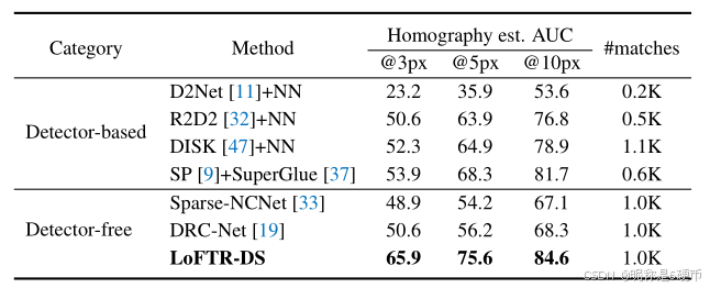
Table 1: Homography estimation on HPatches 7. The AUC of the corner error in percentage is reported. The suffix DS indicates the differentiable matching with dualsoftmax.
Evaluation protocol. In every test sequence, one reference image is paired with the rest five images. All images are resized with shorter dimensions equal to 480. For each image pair, we extract a set of matches with LoFTR trained on MegaDepth 21. We use OpenCV to compute the homography estimation with RANSAC as the robust estimator. To make a fair comparison to methods that produce different numbers of matches, we compute the corner error between the images warped with the estimated H ^ \hat{\mathcal{H}} H^ and the groundtruth H \mathcal{H} H as a correctness identifier as in 9. Following 37, we report the area under the cumulative curve (AUC) of the corner error up to threshold values of 3, 5, and 10 pixels, respectively. We report the results of LoFTR with a maximum of 1K output matches.
【翻译】评估协议。在每个测试序列中,一张参考图像与其余五张图像配对。所有图像的短边被调整为480。对于每对图像,我们使用在MegaDepth 21上训练的LoFTR提取一组匹配。我们使用OpenCV计算单应性估计,RANSAC作为鲁棒估计器。为了与产生不同数量匹配的方法进行公平比较,我们计算使用估计的 H ^ \hat{\mathcal{H}} H^和真实值 H \mathcal{H} H变换后的图像之间的角点误差作为正确性标识符,如9中所述。按照37的方法,我们报告角点误差累积曲线下的面积(AUC),阈值分别为3、5和10像素。我们报告LoFTR最多输出1K个匹配的结果。
Baseline methods. We compare LoFTR with three categories of methods: 1) detector-based local features including R2D2 32, D2Net 11, and DISK 47, 2) a detectorbased local feature matcher, i.e., SuperGlue 37 on top of SuperPoint 9 features, and 3) detector-free matchers including Sparse-NCNet 33 and DRC-Net 19. For local features, we extract a maximum of 2K features with which we extract mutual nearest neighbors as the final matches. For methods directly outputting matches, we restrict a maximum of 1K matches, same as LoFTR. We use the default hyperparameters in the original implementations for all the baselines.
Results. Tab. 1 shows that LoFTR notably outperforms other baselines under all error thresholds by a significant margin. Specifically, the performance gap between LoFTR and other methods increases with a stricter correctness threshold. We attribute the top performance to the larger number of match candidates provided by the detector-free design and the global receptive field brought by the Transformer. Moreover, the coarse-to-fine module also contributes to the estimation accuracy by refining matches to a sub-pixel level.
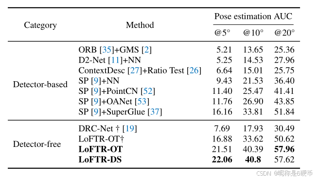
Table 2: Evaluation on ScanNet 7 for indoor pose estimation. The AUC of the pose error in percentage is reported. LoFTR improves the state-of-the-art methods by a large margin. †indicates models trained on MegaDepth. The suffixes OT and DS indicate differentiable matching with optimal transport and dual-softmax, respectively.
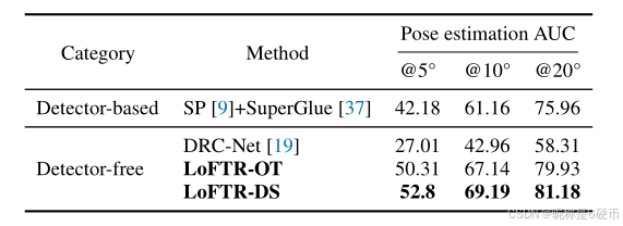
Table 3: Evaluation on MegaDepth 21 for outdoor pose estimation. Matching with LoFTR results in better performance in the outdoor pose estimation task.
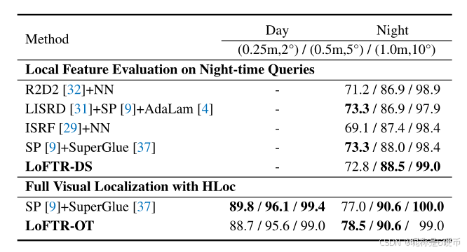
Table 4: Visual localization evaluation on the Aachen Day-Night 54 benchmark v1.1. The evaluation results on both the local feature evaluation track and the full visual localization track are reported.
ScanNet contains 1613 monocular sequences with ground truth poses and depth maps. Following the procedure from SuperGlue 37, we sample 230M image pairs for training, with overlap scores between 0.4 and 0.8. We evaluate our method on the 1500 testing pairs from 37. All images and depth maps are resized to 640 × 480 640\times480 640×480 . This dataset contains image pairs with wide baselines and extensive texture-less regions.
MegaDepth consists of 1M internet images of 196 different outdoor scenes. The authors also provide sparse reconstruction from COLMAP 40 and depth maps computed from multi-view stereo. We follow DISK 47 to only use the scenes of "Sacre Coeur" and "St. Peter's Square" for validation, from which we sample 1500 pairs for a fair comparison. Images are resized such that their longer dimensions are equal to 840 for training and 1200 for validation. The key challenge on MegaDepth is matching under extreme viewpoint changes and repetitive patterns.
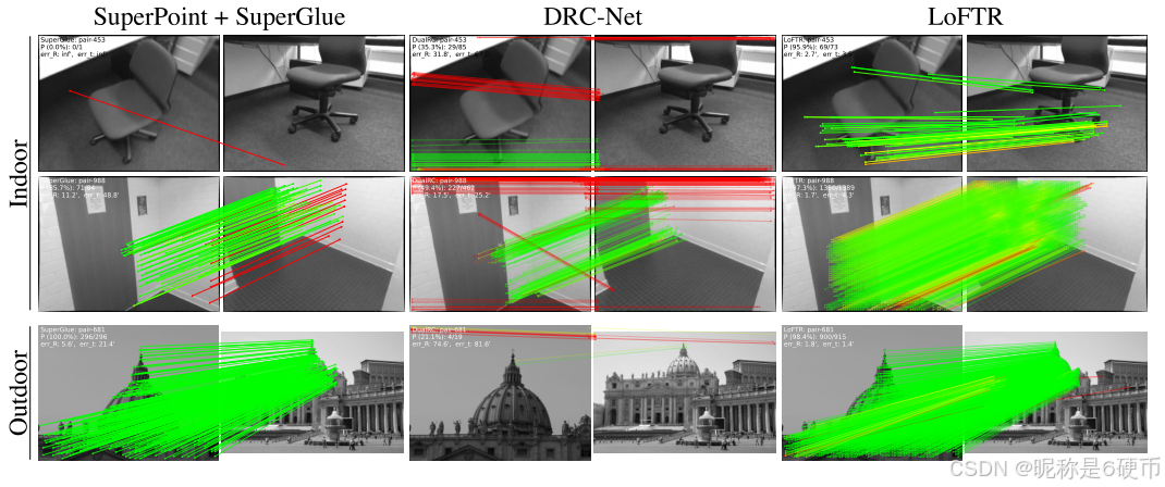
Evaluation protocol. Following 37, we report the AUC of the pose error at thresholds ( 5 ∘ , 10 ∘ , 20 ∘ ) (5^{\circ},10^{\circ},20^{\circ}) (5∘,10∘,20∘) , where the pose error is defined as the maximum of angular error in rotation and translation. To recover the camera pose, we solve the essential matrix from predicted matches with RANSAC. We don't compare the matching precisions between LoFTR and other detector-based methods due to the lack of a well-defined metric (e.g., matching score or recall 13, 30) for detector-free image matching methods. We consider DRCNet 19 as the state-of-the-art method in detector-free approaches 34, 33.
Results of indoor pose estimation. LoFTR achieves the best performance in pose accuracy compared to all competitors (see Tab. 2 and Fig. 5). Pairing LoFTR with optimal transport or dual-softmax as the differentiable matching layer achieves comparable performance. Since the released model of DRC-Net† is trained on MegaDepth, we provide the results of LoFTR† \operatorname{LoFTR\dag} LoFTR† trained on MegaDepth for a fair comparison. LoFTR† \operatorname{LoFTR\dag} LoFTR† also outperforms DRC-Net† by a large margin in this evaluation (see Fig. 5), which demonstrates the generalizability of our model across datasets.
Results of Outdoor Pose Estimation. As shown in Tab. 3, LoFTR outperforms the detector-free method DRC-Net by 61 % 61\% 61% at A U C @ 10 ∘ \operatorname{AUC@10^{\circ}} AUC@10∘ , demonstrating the effectiveness of the Transformer. For SuperGlue, we use the setup from the open-sourced localization toolbox HLoc 36. LoFTR outperforms SuperGlue by a large margin ( 13 % 13\% 13% at A U C @ 10 ∘ ) \operatorname{AUC@10^{\circ}}) AUC@10∘) , which demonstrates the effectiveness of the detector-free design. Different from indoor scenes, LoFTR-DS performs better than LoFTR-OT on MegaDepth. More qualitative results can be found in Fig. 5.
【翻译】室外位姿估计结果。如表3所示,LoFTR在 A U C @ 10 ∘ \operatorname{AUC@10^{\circ}} AUC@10∘上比无检测器方法DRC-Net优越 61 % 61\% 61%,证明了Transformer的有效性。对于SuperGlue,我们使用开源定位工具箱HLoc 36的设置。LoFTR大幅优于SuperGlue(在 A U C @ 10 ∘ \operatorname{AUC@10^{\circ}} AUC@10∘上提升 13 % 13\% 13%),这证明了无检测器设计的有效性。与室内场景不同,LoFTR-DS在MegaDepth上的表现优于LoFTR-OT。更多定性结果可在图5中找到。
4.3. Visual Localization
Visual Localization. Besides achieving competitive performance for relative pose estimation, LoFTR can also benefit visual localization, which is the task to estimate the 6- DoF poses of given images with respect to the corresponding 3D scene model. We evaluate LoFTR on the Long-Term Visual Localization Benchmark 43 (referred to as VisLoc benchmark in the following). It focuses on benchmarking visual localization methods under varying conditions, e.g., day-night changes, scene geometry changes, and indoor scenes with plenty of texture-less areas. Thus, the visual localization task relies on highly robust image matching methods.
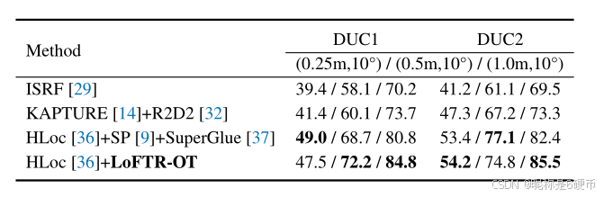
Table 5: Visual localization evaluation on the InLoc 41 benchmark.
【翻译】表5:在InLoc 41基准测试上的视觉定位评估。
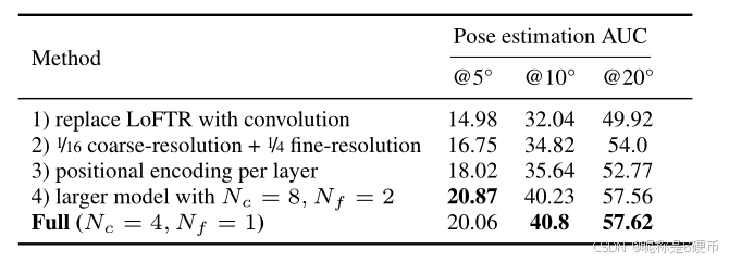
Table 6: Ablation study. Five variants of LoFTR are trained and evaluated both on the ScanNet dataset.
【翻译】表6:消融研究。LoFTR的五个变体都在ScanNet数据集上进行训练和评估。
Evaluation. We evaluate LoFTR on two tracks of VisLoc that consist of several challenges. First, the "visual localization for handheld devices" track requires a full localization pipeline. It benchmarks on two datasets, the AachenDay-Night dataset 38, 54 concerning outdoor scenes and the InLoc 41 dataset concerning indoor scenes. We use open-sourced localization pipeline HLoc 36 with the matches extracted by LoFTR. Second, the "local features for long-term localization" track provides a fixed localization pipeline to evaluate the local feature extractors themselves and optionally the matchers. This track uses the Aachen v1.1 dataset 54. We provide the implementation details of testing LoFTR on VisLoc in the supplementary material.
Results. We provide evaluation results of LoFTR in Tab. 4 and Tab. 5. We have evaluated LoFTR pairing with either the optimal transport layer or the dual-softmax operator and report the one with better results. LoFTR-DS outperforms all baselines in the local feature challenge track, showing its robustness under day-night changes. Then, for the visual localization for handheld devices track, LoFTR-OT outperforms all published methods on the challenging InLoc dataset, which contains extensive appearance changes, more texture-less areas, symmetric and repetitive elements. We attribute the prominence to the use of the Transformer and the optimal transport layer, taking advantage of global information and jointly bringing global consensus into the final matches. The detector-free design also plays a critical role, preventing the repeatability problem of detectorbased methods in low-texture regions. LoFTR-OT performs on par with the state-of-the-art method SuperPoint + SuperGlue on night queries of the Aachen v1.1 dataset and slightly worse on the day queries.
Figure 5: Qualitative results. LoFTR is compared to SuperGlue 37 and DRC-Net 19 in indoor and outdoor environments. LoFTR obtains more correct matches and fewer mismatches, successfully coping with low-texture regions and large viewpoint and illumination changes. The red color indicates epipolar error beyond 5 × 10 − 4 5\times10^{-4} 5×10⁻⁴ for indoor scenes and 1 × 10 − 4 1\times10^{-4} 1×10⁻⁴ for outdoor scenes (in the normalized image coordinates). More qualitative results can be found on the project webpage.
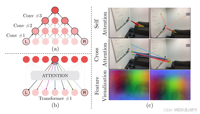
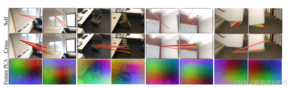
Figure 6: Visualization of self and cross attention weights and the transformed features. In the first two examples, the query point from the low-texture region is able to aggregate the surrounding global information flexibly. For instance, the point on the chair is looking at the edge of the chair. In the last two examples, the query point from the distinctive region can also utilize the richer information from other regions. The feature visualization with PCA further shows that LoFTR learns a position-dependent feature representation.
Ablation Study. To fully understand the different modules in LoFTR, we evaluate five different variants with results shown in Tab. 6: 1) Replacing the LoFTR module by convolution with a comparable number of parameters results in a significant drop in AUC as expected. 2) Using a smaller version of LoFTR with 1 / 16 1/16 1/16 and 1 / 4 1/4 1/4 resolution feature maps at the coarse and fine level, respectively, results in a running time of 104 m s 104~\mathrm{{ms}} 104 ms and a degraded pose estimation accuracy. 3) Using DETR-style 3 Transformer architecture which has positional encoding at each layer, leads to a noticeably declined result. 4) Increasing the model capacity by doubling the number of LoFTR layers to N c = 8 N_{c}=8 Nc=8 and N f = 2 N_{f}=2 Nf=2 barely changes the results. We conduct these experiments using the same training and evaluation protocol as indoor pose estimation on ScanNet with an optimal transport layer for matching.
【翻译】消融研究。为了充分理解LoFTR中的不同模块,我们评估了五个不同的变体,结果如表6所示:1)用具有相当参数数量的卷积替换LoFTR模块会导致AUC显著下降,这在预期之中。2)使用较小版本的LoFTR,在粗粒度和细粒度级别分别使用 1 / 16 1/16 1/16和 1 / 4 1/4 1/4分辨率的特征图,导致运行时间为 104 m s 104~\mathrm{{ms}} 104 ms且位姿估计精度下降。3)使用DETR风格3的Transformer架构(每层都有位置编码)会导致结果明显下降。4)通过将LoFTR层数加倍至 N c = 8 N_{c}=8 Nc=8和 N f = 2 N_{f}=2 Nf=2来增加模型容量几乎不会改变结果。我们使用与ScanNet上室内位姿估计相同的训练和评估协议进行这些实验,并使用最优传输层进行匹配。
Visualizing Attention. We visualize the attention weights in Fig. 6.
【翻译】注意力可视化。我们在图6中可视化了注意力权重。
5. Conclusion
This paper presents a novel detector-free matching approach, named LoFTR, that can establish accurate semidense matches with Transformers in a coarse-to-fine manner. The proposed LoFTR module uses the self and cross attention layers in Transformers to transform the local features to be context- and position-dependent, which is crucial for LoFTR to obtain high-quality matches on indistinctive regions with low-texture or repetitive patterns. Our experiments show that LoFTR achieves state-of-the-art performances on relative pose estimation and visual localization on multiple datasets. We believe that LoFTR provides a new direction for detector-free methods in local image feature matching and can be extended to more challenging scenarios, e.g., matching images with severe seasonal changes.