评估指标：AP（Average Precision）、mAP（Mean Average Precision）

评估指标：AP（Average Precision）、mAP（Mean Average Precision）

• 前言
• 相关介绍
• • • [AP（Average Precision）](#AP（Average Precision）)
    • [mAP（Mean Average Precision）](#mAP（Mean Average Precision）)
    • 注意事项
• [AP（Average Precision）](#AP（Average Precision）)
• • [近似 AP（approximated average precision）](#近似 AP（approximated average precision）)
  • • 计算实例
  • 代码示例
  • • Python实现
  • [插值 AP（Interpolated average precision）](#插值 AP（Interpolated average precision）)
  • • 计算实例
    • • 示例数据
      • 插值计算步骤
      • • 插值示例：
  • 代码示例
  • • Python实现
  • 完整代码
• 参考

前言

• 由于本人水平有限，难免出现错漏，敬请批评改正。
• 更多精彩内容，可点击进入Python日常小操作专栏、OpenCV-Python小应用专栏、YOLO系列专栏、自然语言处理专栏、人工智能混合编程实践专栏或我的个人主页查看
• YOLOs-CPP：一个免费开源的YOLO全系列C++推理库（以YOLO26为例）
• PaddleOCR：Win10上安装使用PPOCRLabel标注工具
• 目标检测：使用自己的数据集微调DEIMv2进行物体检测
• 图像分割：PyTorch从零开始实现SegFormer语义分割
• 图像超分：使用自己的数据集微调Real-ESRGAN-x4plus进行超分重建
• 图像生成：PyTorch从零开始实现一个简单的扩散模型
• Stable Diffusion：使用自己的数据集微调 Stable Diffusion 3.5 LoRA 文生图模型
• 图像超分：使用自己的数据集微调Real-ESRGAN-x2plus进行超分重建
• Anomalib：使用Anomalib 2.1.0训练自己的数据集进行异常检测
• Anomalib：在Linux服务器上安装使用Anomalib 2.1.0
• 人工智能混合编程实践：C++调用封装好的DLL进行异常检测推理
• 人工智能混合编程实践：C++调用封装好的DLL进行FP16图像超分重建（v3.0）
• 隔离系统Python：源码编译3.11.8到自定义目录（含PGO性能优化）
• 在线机的Python环境迁移到离线机上
• Nuitka 将 Python 脚本封装为 .pyd 或 .so 文件
• Ultralytics：使用 YOLO11 进行速度估计
• Ultralytics：使用 YOLO11 进行物体追踪
• Ultralytics：使用 YOLO11 进行物体计数
• Ultralytics：使用 YOLO11 进行目标打码
• 人工智能混合编程实践：C++调用Python ONNX进行YOLOv8推理
• 人工智能混合编程实践：C++调用封装好的DLL进行YOLOv8实例分割
• 人工智能混合编程实践：C++调用Python ONNX进行图像超分重建
• 人工智能混合编程实践：C++调用Python AgentOCR进行文本识别
• 通过计算实例简单地理解PatchCore异常检测
• Python将YOLO格式实例分割数据集转换为COCO格式实例分割数据集
• YOLOv8 Ultralytics：使用Ultralytics框架训练RT-DETR实时目标检测模型
• 基于DETR的人脸伪装检测
• YOLOv7训练自己的数据集（口罩检测）
• YOLOv8训练自己的数据集（足球检测）
• YOLOv5：TensorRT加速YOLOv5模型推理
• YOLOv5：IoU、GIoU、DIoU、CIoU、EIoU
• 玩转Jetson Nano（五）：TensorRT加速YOLOv5目标检测
• YOLOv5：添加SE、CBAM、CoordAtt、ECA注意力机制
• YOLOv5：yolov5s.yaml配置文件解读、增加小目标检测层
• Python将COCO格式实例分割数据集转换为YOLO格式实例分割数据集
• YOLOv5：使用7.0版本训练自己的实例分割模型（车辆、行人、路标、车道线等实例分割）
• 使用Kaggle GPU资源免费体验Stable Diffusion开源项目
• Stable Diffusion：在服务器上部署使用Stable Diffusion WebUI进行AI绘图（v2.0）
• Stable Diffusion：使用自己的数据集微调训练LoRA模型（v2.0）

相关介绍

AP 衡量的是训练好的模型在每个类别上的好坏，mAP 衡量的是模型在所有类别上的好坏，得到 AP 后 mAP 的计算就变得很简单了，就是取所有 AP 的平均值。AP 的计算公式比较复杂（所以单独作一章节内容），详细内容参考下文。

mAP 这个术语有不同的定义。此度量指标通常用于信息检索、图像分类和目标检测领域。然而这两个领域计算 mAP 的方式却不相同。这里我们只谈论目标检测中的 mAP 计算方法。

mAP 常作为目标检测算法的评价指标，具体来说就是，对于每张图片检测模型会输出多个预测框（远超真实框的个数），我们使用 IoU (Intersection Over Union，交并比)来标记预测框是否预测准确。标记完成后，随着预测框的增多，查全率 R 总会上升，在不同查全率 R 水平下对准确率 P 做平均，即得到 AP ，最后再对所有类别按其所占比例做平均，即得到 mAP 指标。

AP（Average Precision）

定义 ：

AP，即平均精度，是在目标检测或信息检索等领域中用于衡量模型在单个类别上的性能。它通过计算不同召回率（Recall）水平下的精确率（Precision）的平均值来衡量模型的精度。在计算AP时，通常会生成一个PR曲线（Precision-Recall曲线），该曲线上的点表示不同召回率下模型的精确率。AP即为PR曲线下方的面积。

公式 :

理论上可以通过积分来计算AP，公式如下：
A P = ∫ 0 1 P ( r ) d r AP=\int_0^1 P(r) dr AP=∫01P(r)dr

但通常情况下都是使用近似或者插值的方法来计算 A P AP AP。

A P = ∑ k = 1 N P ( k ) Δ r ( k ) AP = \sum_{k=1}^{N}P(k)\Delta r(k) AP=k=1∑NP(k)Δr(k)

• 近似计算 A P AP AP (approximated average precision)，这种计算方式是 approximated 形式的；
• 很显然位于一条竖直线上的点对计算 A P AP AP 没有贡献；
• 这里 N N N 为数据总量， k k k 为每个样本点的索引， Δ r ( k ) = r ( k ) − r ( k − 1 ) Δr(k)=r(k)−r(k−1) Δr(k)=r(k)−r(k−1)。

插值计算(Interpolated average precision) A P AP AP 的公式：

• 这是通常意义上的 11 points_Interpolated 形式的 AP，选取固定的 0 , 0.1 , 0.2 , ... , 1.0 , {0,0.1,0.2,...,1.0}, 0,0.1,0.2,...,1.0, 11 个阈值，这个在 PASCAL2007 中使用
• 这里因为参与计算的只有 11 个点，所以 K = 11 K=11 K=11，称为 11 points_Interpolated， k k k 为阈值索引
• P i n t e r p ( k ) P_{interp}(k) Pinterp(k) 取第 k k k 个阈值所对应的样本点之后的样本中的最大值，只不过这里的阈值被限定在了 0 , 0.1 , 0.2 , ... , 1.0 {0,0.1,0.2,...,1.0} 0,0.1,0.2,...,1.0 范围内。

优缺点:

• 优点：

  • 能够全面反映模型在不同召回率水平下的精确率表现，适用于类别不平衡的数据。
  • PR曲线直观展示模型性能，AP作为其积分，具有较好的解释性。

• 缺点：

  • 计算相对复杂，尤其是在处理大量预测结果时。
  • 对极端情况（如单一预测框的召回率和精确率）敏感，可能导致波动较大。

mAP（Mean Average Precision）

定义 ：

mAP，即平均平均精度，是目标检测任务中常用的综合评价指标，它通过对所有类别分别计算AP，然后取这些AP的平均值来评估模型的整体性能。这使得mAP能够反映模型在多类别分类和定位任务中的综合能力。

公式 :
m A P = 1 C ∑ c = 1 C A P c mAP = \frac{1}{C} \sum_{c=1}^{C} AP_c mAP=C1c=1∑CAPc

其中， C C C 是类别总数， A P c AP_c APc是第(c)个类别的AP值。

优缺点:

• 优点：

  • 提供了一个统一的标准来衡量多类别检测任务的性能。
  • 能够综合考虑所有类别的检测效果，适用于评估模型在复杂环境下的表现。

• 缺点：

  • 平均操作可能会掩盖某些类别表现不佳的问题，尤其是当类别之间性能差异很大时。
  • 对类别不平衡敏感，如果某些类别样本数量极少，其AP可能对mAP的贡献较小或产生偏差。

注意事项

• 在计算AP和mAP时，通常会使用交并比（IoU，Intersection over Union）来确定预测框与真实框之间的匹配程度，常见的阈值为0.5。
• 为了更公平地比较不同模型，确保在相同的IoU阈值和评估策略（如是否考虑难样本）下进行评估。
• 在实践中，mAP的计算还会涉及到一些细节，如非极大值抑制（NMS）的应用，以及对预测框的排序规则等。

AP（Average Precision）

近似 AP（approximated average precision）

A P = ∑ k = 1 N P ( k ) Δ r ( k ) AP = \sum_{k=1}^{N}P(k)\Delta r(k) AP=k=1∑NP(k)Δr(k)

• 近似计算 A P AP AP (approximated average precision)，这种计算方式是 approximated 形式的；
• 很显然位于一条竖直线上的点对计算 A P AP AP 没有贡献；
• 这里 N N N 为数据总量， k k k 为每个样本点的索引， Δ r ( k ) = r ( k ) − r ( k − 1 ) Δr(k)=r(k)−r(k−1) Δr(k)=r(k)−r(k−1)。

计算实例

为了近似计算AP（Average Precision）的一个实例，我们可以简化过程并手动走一遍计算流程。假设我们有一个二分类问题，并且得到了以下关于某个类别的预测结果和它们与真实标签的对应情况（为了简化，我们只列出了一些关键点）：

预测序号	预测分数	是否为正类 (P/T)	是否被正确预测 (C/T)
1	0.9	T	T
2	0.8	F	F
3	0.7	T	F
4	0.6	T	T
5	0.5	F	F
6	0.4	T	T

在这个例子中，"是否为正类 (P/T)" 列表明该预测是属于正类（Positive）还是负类（Negative）；"是否被正确预测 (C/T)" 列表明预测是否正确。

步骤:

1. 排序：首先，按照预测分数从高到低排序（在这个简化示例中，已经按分数排列）。

2. 计算精确率 (Precision) 和召回率 (Recall)：遍历列表，每次增加一个预测结果，更新精确率和召回率。

   • 精确率 = TP / (TP + FP)，其中TP是真正例(True Positive)，FP是假正例(False Positive)。
   • 召回率 = TP / (TP + FN)，其中FN是假负例(False Negative)。

3. 计算AP：通过插值法或直接计算每个召回率点对应的精确率，然后计算曲线下方的面积。

手动计算：

• 当考虑前1个预测时，没有召回率变化（因为还没有假负例），所以不计算AP。
• 考虑前2个预测，召回率为0/2=0，不计算AP。
• 考虑前3个预测，召回率变为1/3，精确率也是1/3，但不直接计算AP点。
• 考虑前4个预测，召回率变为2/4=0.5，精确率变为2/4=0.5，得到一个(0.5, 0.5)的点。
• 考虑所有预测，最终召回率为3/4=0.75，精确率为3/6=0.5。

近似计算：

• 假设不进行插值，仅考虑这些关键点，我们的AP近似计算基于这些点。但由于我们只有两个有效点(0.5, 0.5)和(0.75, 0.5)，可以简单地认为AP为这两个点形成的矩形的一半（因为曲线在此处假设是水平的）。

A P ≈ ( 0.75 − 0.5 ) ∗ 0.5 2 = 0.25 ∗ 0.5 2 = 0.125 2 = 0.0625 AP \approx \frac{(0.75-0.5) * 0.5}{2} = \frac{0.25 * 0.5}{2} = \frac{0.125}{2} = 0.0625 AP≈2(0.75−0.5)∗0.5=20.25∗0.5=20.125=0.0625

这个是非常简化的计算，实际计算AP时，通常会在多个召回率点上计算精确率，且会采用插值法使曲线平滑，从而更准确地计算AP的积分值。上述示例仅仅是为了说明基本概念，并未严格遵循插值法或考虑所有可能的精确率-召回率点组合。

代码示例

Python实现

import numpy as np

def sort_by_scores(y_true, y_scores):
    """按预测分数排序真实标签和预测概率"""
    order = np.argsort(y_scores)[::-1]
    return y_true[order], y_scores[order]

# 示例数据
y_true = np.array([0, 1, 1, 1, 0, 1])  # 真实标签
y_scores = np.array([0.1, 0.4, 0.35, 0.8, 0.6, 0.9])  # 预测概率

y_true_sorted, y_scores_sorted = sort_by_scores(y_true, y_scores)

def approximate_AP(precision, recall):
    """近似计算AP"""
    # 累积精确率的和作为AP的近似值
    return np.sum((recall[1:] - recall[:-1]) * precision[1:])

def calculate_precision_recall(y_true, y_scores):
    """计算精确率和召回率"""
    n_positives = np.sum(y_true == 1)
    n_negatives = np.sum(y_true == 0)
    
    precision = np.cumsum(y_true == 1) / (np.arange(len(y_true)) + 1)
    recall = np.cumsum(y_true == 1) / n_positives
    
    # 处理最后一个点，确保召回率为1时的精确率正确
    if n_positives > 0:
        precision[-1] = np.sum(y_true == 1) / np.sum(y_scores >= y_scores[-1])
    else:
        precision = np.zeros_like(recall)
    
    return precision, recall

precision, recall = calculate_precision_recall(y_true_sorted, y_scores_sorted)
print([(x,y) for y,x in zip(precision, recall)]) # [(0.25, 1.0), (0.5, 1.0), (0.5, 0.6666666666666666), (0.75, 0.75), (1.0, 0.8), (1.0, 0.6666666666666666)]
approx_ap = approximate_AP(precision, recall)
print(f"近似AP: {approx_ap}") # 近似AP: 0.6375

插值 AP（Interpolated average precision）

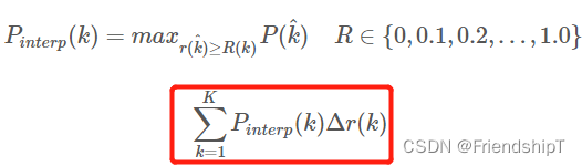
插值计算(Interpolated average precision) A P AP AP 的公式：

• 这是通常意义上的 11 points_Interpolated 形式的 AP，选取固定的 0 , 0.1 , 0.2 , ... , 1.0 , {0,0.1,0.2,...,1.0}, 0,0.1,0.2,...,1.0, 11 个阈值，这个在 PASCAL2007 中使用
• 这里因为参与计算的只有 11 个点，所以 K = 11 K=11 K=11，称为 11 points_Interpolated， k k k 为阈值索引
• P i n t e r p ( k ) P_{interp}(k) Pinterp(k) 取第 k k k 个阈值所对应的样本点之后的样本中的最大值，只不过这里的阈值被限定在了 0 , 0.1 , 0.2 , ... , 1.0 {0,0.1,0.2,...,1.0} 0,0.1,0.2,...,1.0 范围内。

计算实例

插值计算AP（Average Precision）是一种更精确的方法，用于计算PR曲线（Precision-Recall Curve）下的面积，以评估模型的性能。下面通过一个简化的实例来说明插值法如何应用于AP的计算：

示例数据

假设我们有一个二分类任务的预测结果，针对某一类别，按预测分数降序排列后，得到如下数据（简化版，只列出关键点）：

预测编号	预测分数	是否为正类 (P/T)	是否正确 (C/T)	累积TP	累积FP	精确率	召回率
1	0.9	T	T	1	0	1.00	1.00
2	0.8	F	F	1	1	0.50	1.00
3	0.7	T	F	1	2	0.33	0.50
4	0.6	T	T	2	2	0.50	1.00
5	0.5	F	F	2	3	0.40	0.66
6	0.4	T	T	3	3	0.50	1.00

插值计算步骤

1. 计算精确率和召回率：如上表所示，随着每一个预测结果的加入，累积计算TP（真正例）、FP（假正例），进而计算精确率和召回率。

2. 确定召回率点：为了进行插值，我们首先确定PR曲线上的召回率点。假设我们关心的召回率点为0, 0.25, 0.5, 0.75, 1。注意，实际应用中这些点通常是根据实际数据点间插值得到的。

3. 插值计算：对于每个召回率点，找到最接近该召回率的两个真实召回率点，并在这两点间进行线性插值，以估算该召回率对应的精确率。

插值示例：

• 召回率0.5：在我们的数据中，直接有召回率0.5的情况，对应的精确率为0.50。

• 召回率0.75：最近的两个点是召回率0.66和1.00，对应精确率分别是0.40和0.50。进行线性插值计算精确率。

  插值公式可以简化为：
  P i n t e r p = P l o w e r + ( R e c a l l t a r g e t − R e c a l l l o w e r ) ( R e c a l l u p p e r − R e c a l l l o w e r ) × ( P u p p e r − P l o w e r ) P_{interp} = P_{lower} + \frac{(Recall_{target} - Recall_{lower})}{(Recall_{upper} - Recall_{lower})} \times (P_{upper} - P_{lower}) Pinterp=Plower+(Recallupper−Recalllower)(Recalltarget−Recalllower)×(Pupper−Plower)

  其中，(P_{interp})是要插值得到的精确率，(P_{lower}, P_{upper})分别是召回率低于和高于目标召回率的精确率值，(Recall_{lower}, Recall_{upper})对应的是这两个精确率的召回率值，(Recall_{target})是我们要插值的目标召回率。

  代入数据计算召回率为0.75时的精确率：
  P i n t e r p = 0.40 + ( 0.75 − 0.66 ) ( 1.00 − 0.66 ) × ( 0.50 − 0.40 ) = 0.40 + 0.09 0.34 × 0.10 ≈ 0.40 + 0.0265 = 0.4265 P_{interp} = 0.40 + \frac{(0.75 - 0.66)}{(1.00 - 0.66)} \times (0.50 - 0.40) = 0.40 + \frac{0.09}{0.34} \times 0.10 \approx 0.40 + 0.0265 = 0.4265 Pinterp=0.40+(1.00−0.66)(0.75−0.66)×(0.50−0.40)=0.40+0.340.09×0.10≈0.40+0.0265=0.4265

4. 计算AP：将所有插值计算得到的精确率乘以相邻召回率差值，然后求和。因为我们的示例比较简单，实际操作中会根据更多插值点进行计算。但基于简化数据，我们仅展示了召回率为0.5和0.75的处理方法，完整计算需覆盖所有指定召回率点。

注意，实际应用中，插值过程通常由评估软件自动完成，如在使用sklearn.metrics.average_precision_score函数时，会自动进行这些复杂的计算，直接给出AP值。

代码示例

Python实现

import numpy as np

def sort_by_scores(y_true, y_scores):
    """按预测分数排序真实标签和预测概率"""
    order = np.argsort(y_scores)[::-1]
    return y_true[order], y_scores[order]

# 示例数据
y_true = np.array([0, 1, 1, 1, 0, 1])  # 真实标签
y_scores = np.array([0.1, 0.4, 0.35, 0.8, 0.6, 0.9])  # 预测概率

y_true_sorted, y_scores_sorted = sort_by_scores(y_true, y_scores)

def calculate_precision_recall(y_true, y_scores):
    """计算精确率和召回率"""
    n_positives = np.sum(y_true == 1)
    n_negatives = np.sum(y_true == 0)
    
    precision = np.cumsum(y_true == 1) / (np.arange(len(y_true)) + 1)
    recall = np.cumsum(y_true == 1) / n_positives
    
    # 处理最后一个点，确保召回率为1时的精确率正确
    if n_positives > 0:
        precision[-1] = np.sum(y_true == 1) / np.sum(y_scores >= y_scores[-1])
    else:
        precision = np.zeros_like(recall)
    
    return precision, recall

precision, recall = calculate_precision_recall(y_true_sorted, y_scores_sorted)
print([(x,y) for y,x in zip(precision, recall)]) # [(0.25, 1.0), (0.5, 1.0), (0.5, 0.6666666666666666), (0.75, 0.75), (1.0, 0.8), (1.0, 0.6666666666666666)]

def interpolated_AP(precision, recall):
    """插值计算AP"""
    recall = np.concatenate([[0.], recall, [1.]])  # 在两端添加0和1
    precision = np.concatenate([[0.], precision, [precision[-1]]])  # 末尾复制精确率值
    # 对召回率排序并对应地排序精确率
    indices = np.argsort(recall)
    recall = recall[indices]
    precision = precision[indices]
    
    # 计算斜率并进行插值
    for i in range(1, len(precision) - 1, 3):  # 跳过端点，每三个点考虑一次
        if precision[i+1] < precision[i]:
            precision[i+1:] = np.maximum(precision[i], precision[i+1:])
    
    # 插值后计算AP
    ap = np.trapz(precision, recall)
    return ap

interp_ap = interpolated_AP(precision, recall)
print(f"插值计算AP: {interp_ap}") # 插值计算AP: 0.7458333333333332

完整代码

def sort_by_scores(y_true, y_scores):
    """按预测分数排序真实标签和预测概率"""
    order = np.argsort(y_scores)[::-1]
    return y_true[order], y_scores[order]

# 示例数据
y_true = np.array([0, 1, 1, 1, 0, 1])  # 真实标签
y_scores = np.array([0.1, 0.4, 0.35, 0.8, 0.6, 0.9])  # 预测概率

y_true_sorted, y_scores_sorted = sort_by_scores(y_true, y_scores)

def approximate_AP(precision, recall):
    """近似计算AP"""
    # 累积精确率的和作为AP的近似值
    return np.sum((recall[1:] - recall[:-1]) * precision[1:])

def calculate_precision_recall(y_true, y_scores):
    """计算精确率和召回率"""
    n_positives = np.sum(y_true == 1)
    n_negatives = np.sum(y_true == 0)
    
    precision = np.cumsum(y_true == 1) / (np.arange(len(y_true)) + 1)
    recall = np.cumsum(y_true == 1) / n_positives
    
    # 处理最后一个点，确保召回率为1时的精确率正确
    if n_positives > 0:
        precision[-1] = np.sum(y_true == 1) / np.sum(y_scores >= y_scores[-1])
    else:
        precision = np.zeros_like(recall)
    
    return precision, recall

precision, recall = calculate_precision_recall(y_true_sorted, y_scores_sorted)
print([(x,y) for y,x in zip(precision, recall)])
approx_ap = approximate_AP(precision, recall)
print(f"近似AP: {approx_ap}")

def interpolated_AP(precision, recall):
    """插值计算AP"""
    recall = np.concatenate([[0.], recall, [1.]])  # 在两端添加0和1
    precision = np.concatenate([[0.], precision, [precision[-1]]])  # 末尾复制精确率值
    # 对召回率排序并对应地排序精确率
    indices = np.argsort(recall)
    recall = recall[indices]
    precision = precision[indices]
    
    # 计算斜率并进行插值
    for i in range(1, len(precision) - 1, 3):  # 跳过端点，每三个点考虑一次
        if precision[i+1] < precision[i]:
            precision[i+1:] = np.maximum(precision[i], precision[i+1:])
    
    # 插值后计算AP
    ap = np.trapz(precision, recall)
    return ap

interp_ap = interpolated_AP(precision, recall)
print(f"插值计算AP: {interp_ap}")

import matplotlib.pyplot as plt

plt.figure(figsize=(10, 6))
plt.plot(recall, precision, marker='o', label=f'PR Curve (Approx. AP={approx_ap:.3f}, Interp. AP={interp_ap:.3f})')
plt.xlabel('Recall')
plt.ylabel('Precision')
plt.title('Precision-Recall Curve')
plt.legend()
plt.grid(True)
plt.show()

[(0.25, 1.0), (0.5, 1.0), (0.5, 0.6666666666666666), (0.75, 0.75), (1.0, 0.8), (1.0, 0.6666666666666666)]
近似AP: 0.6375
插值计算AP: 0.7458333333333332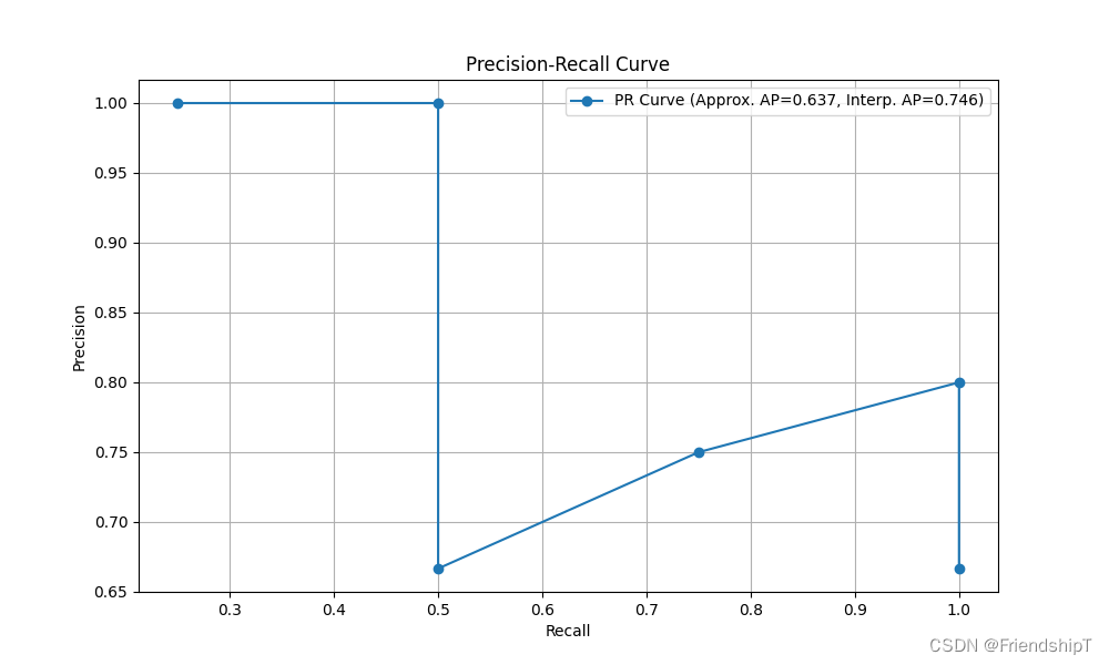

参考

1\] https://github.com/HarleysZhang/cv_note > * 由于本人水平有限，难免出现错漏，敬请批评改正。 > * 更多精彩内容，可点击进入[Python日常小操作](https://blog.csdn.net/friendshiptang/category_11653584.html)专栏、[OpenCV-Python小应用](https://blog.csdn.net/friendshiptang/category_11975851.html)专栏、[YOLO系列](https://blog.csdn.net/friendshiptang/category_12168736.html)专栏、[自然语言处理](https://blog.csdn.net/friendshiptang/category_12396029.html)专栏、[人工智能混合编程实践](https://blog.csdn.net/friendshiptang/category_12915912.html)专栏或我的[个人主页](https://blog.csdn.net/FriendshipTang)查看 > * [YOLOs-CPP：一个免费开源的YOLO全系列C++推理库（以YOLO26为例）](https://blog.csdn.net/FriendshipTang/article/details/158886725) > * [PaddleOCR：Win10上安装使用PPOCRLabel标注工具](https://blog.csdn.net/FriendshipTang/article/details/156572297) > * [目标检测：使用自己的数据集微调DEIMv2进行物体检测](https://blog.csdn.net/FriendshipTang/article/details/153635354) > * [图像分割：PyTorch从零开始实现SegFormer语义分割](https://blog.csdn.net/FriendshipTang/article/details/152268871) > * [图像超分：使用自己的数据集微调Real-ESRGAN-x4plus进行超分重建](https://blog.csdn.net/FriendshipTang/article/details/153331274) > * [图像生成：PyTorch从零开始实现一个简单的扩散模型](https://blog.csdn.net/FriendshipTang/article/details/154358228) > * [Stable Diffusion：使用自己的数据集微调 Stable Diffusion 3.5 LoRA 文生图模型](https://blog.csdn.net/FriendshipTang/article/details/153737733) > * [图像超分：使用自己的数据集微调Real-ESRGAN-x2plus进行超分重建](https://blog.csdn.net/FriendshipTang/article/details/153314081) > * [Anomalib：使用Anomalib 2.1.0训练自己的数据集进行异常检测](https://blog.csdn.net/FriendshipTang/article/details/150561799) > * [Anomalib：在Linux服务器上安装使用Anomalib 2.1.0](https://blog.csdn.net/FriendshipTang/article/details/150499849) > * [人工智能混合编程实践：C++调用封装好的DLL进行异常检测推理](https://blog.csdn.net/FriendshipTang/article/details/153200335) > * [人工智能混合编程实践：C++调用封装好的DLL进行FP16图像超分重建（v3.0）](https://blog.csdn.net/FriendshipTang/article/details/154637411) > * [隔离系统Python：源码编译3.11.8到自定义目录（含PGO性能优化）](https://blog.csdn.net/FriendshipTang/article/details/154641702) > * [在线机的Python环境迁移到离线机上](https://blog.csdn.net/FriendshipTang/article/details/151580480) > * [Nuitka 将 Python 脚本封装为 .pyd 或 .so 文件](https://blog.csdn.net/FriendshipTang/article/details/151617965) > * [Ultralytics：使用 YOLO11 进行速度估计](https://blog.csdn.net/FriendshipTang/article/details/151989345) > * [Ultralytics：使用 YOLO11 进行物体追踪](https://blog.csdn.net/FriendshipTang/article/details/151988142) > * [Ultralytics：使用 YOLO11 进行物体计数](https://blog.csdn.net/FriendshipTang/article/details/151866467) > * [Ultralytics：使用 YOLO11 进行目标打码](https://blog.csdn.net/FriendshipTang/article/details/151868450) > * [人工智能混合编程实践：C++调用Python ONNX进行YOLOv8推理](https://blog.csdn.net/FriendshipTang/article/details/146188546) > * [人工智能混合编程实践：C++调用封装好的DLL进行YOLOv8实例分割](https://blog.csdn.net/FriendshipTang/article/details/149050653) > * [人工智能混合编程实践：C++调用Python ONNX进行图像超分重建](https://blog.csdn.net/FriendshipTang/article/details/146210258) > * [人工智能混合编程实践：C++调用Python AgentOCR进行文本识别](https://blog.csdn.net/FriendshipTang/article/details/146336798) > * [通过计算实例简单地理解PatchCore异常检测](https://blog.csdn.net/FriendshipTang/article/details/148877810) > * [Python将YOLO格式实例分割数据集转换为COCO格式实例分割数据集](https://blog.csdn.net/FriendshipTang/article/details/149101072) > * [YOLOv8 Ultralytics：使用Ultralytics框架训练RT-DETR实时目标检测模型](https://blog.csdn.net/FriendshipTang/article/details/132498898) > * [基于DETR的人脸伪装检测](https://blog.csdn.net/FriendshipTang/article/details/131670277) > * [YOLOv7训练自己的数据集（口罩检测）](https://blog.csdn.net/FriendshipTang/article/details/126513426) > * [YOLOv8训练自己的数据集（足球检测）](https://blog.csdn.net/FriendshipTang/article/details/129035180) > * [YOLOv5：TensorRT加速YOLOv5模型推理](https://blog.csdn.net/FriendshipTang/article/details/131023963) > * [YOLOv5：IoU、GIoU、DIoU、CIoU、EIoU](https://blog.csdn.net/FriendshipTang/article/details/129969044) > * [玩转Jetson Nano（五）：TensorRT加速YOLOv5目标检测](https://blog.csdn.net/FriendshipTang/article/details/126696542) > * [YOLOv5：添加SE、CBAM、CoordAtt、ECA注意力机制](https://blog.csdn.net/FriendshipTang/article/details/130396540) > * [YOLOv5：yolov5s.yaml配置文件解读、增加小目标检测层](https://blog.csdn.net/FriendshipTang/article/details/130375883) > * [Python将COCO格式实例分割数据集转换为YOLO格式实例分割数据集](https://blog.csdn.net/FriendshipTang/article/details/131979248) > * [YOLOv5：使用7.0版本训练自己的实例分割模型（车辆、行人、路标、车道线等实例分割）](https://blog.csdn.net/FriendshipTang/article/details/131987249) > * [使用Kaggle GPU资源免费体验Stable Diffusion开源项目](https://blog.csdn.net/FriendshipTang/article/details/132238734) > * [Stable Diffusion：在服务器上部署使用Stable Diffusion WebUI进行AI绘图（v2.0）](https://blog.csdn.net/FriendshipTang/article/details/150287538) > * [Stable Diffusion：使用自己的数据集微调训练LoRA模型（v2.0）](https://blog.csdn.net/FriendshipTang/article/details/150283800)