机器学习笔记一

摘要

本周回顾了线性模型的基本概念以及训练方法，并进行代码实操。从设立模型开始并进行optimization，经过50轮的运行得到最终结果。

abstract

This week, we reviewed the basic concepts of linear models and training methods, and conducted hands-on coding practice. We started by setting up the model and performing optimization, and after 50 rounds of running, we obtained the final results.

一、线性模型

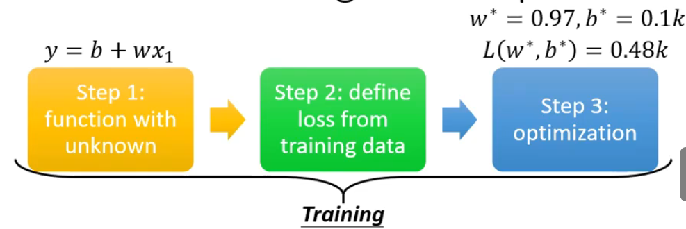
线性模型是一种假设输出与输入特征之间存在线性关系的机器学习模型。就是用一条直线来拟合数据。模型的训练方法如下图所示

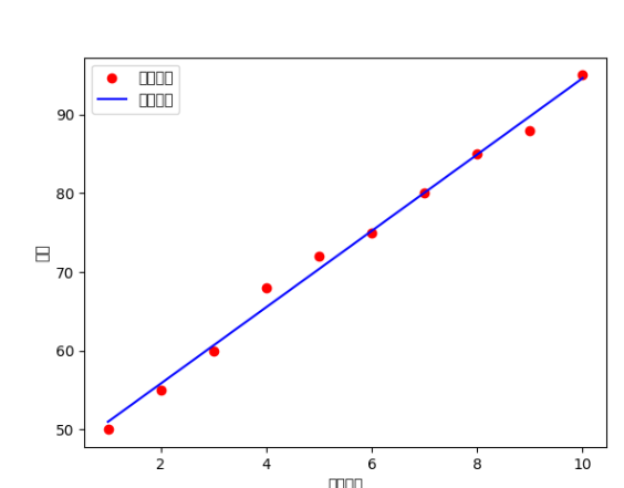
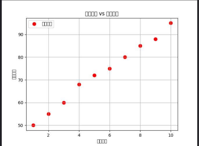
本次的数据集为学习时长[1, 2, 3, 4, 5, 6, 7, 8, 9, 10]与考试分数[50, 55, 60, 68, 72, 75, 80, 85, 88, 95]。

python 复制代码

# X：学习时长
X = np.array([1, 2, 3, 4, 5, 6, 7, 8, 9, 10])
# y：考试分数
y = np.array([50, 55, 60, 68, 72, 75, 80, 85, 88, 95])

二、训练

二.1 、初始化参数

根据数据集的数据分布情况可以初步推断学习时长与考试分数之间存在线性关系因此设:**y=wX+b。**初始斜率以及截距为0，每次更新的步幅为0.1，训练50次停止。选择MSE用于计算loss

python 复制代码

w = 0.0    # 斜率：初始=0
b = 0.0    # 截距：初始=0
lr = 0.1   # 学习率：每次更新的步长
epochs = 50  # 训练 50 次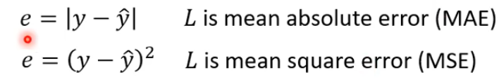

二.2、训练

1step，将X带入到模型中得到预测值y_pred

python 复制代码

y_pred = w * X_norm + b

2step,计算loss =

python 复制代码

loss = np.mean((y_pred - y_norm) ** 2)

3step，optimization

首先求解loss对w的偏微分及及对（y-y_pred）^2进行求导，其中y视为常数。同理可得db

python 复制代码

dw = np.mean(2 * X_norm * (y_pred - y_norm))
db = np.mean(2 * (y_pred - y_norm))

进行更新

python 复制代码

w = w - lr * dw
b = b - lr * db

三，实验结果

经过50轮的更新得到：y = 4.85 × X + 46.13