基于 PyTorch + sklearn 的房价预测实战

House Price Prediction with PyTorch + sklearn (Bilingual Guide)

本文实现了一个完整的房价预测流程，融合了 sklearn 的特征工程与 PyTorch 的神经网络建模。

This article implements a complete house price prediction pipeline combining sklearn feature engineering and PyTorch modeling.

整体流程包括：数据预处理、特征工程、模型训练以及结果可视化。

The workflow includes data preprocessing, feature engineering, model training, and visualization.

使用House Prices数据集：https://www.kaggle.com/c/house-prices-advanced-regression-techniques。

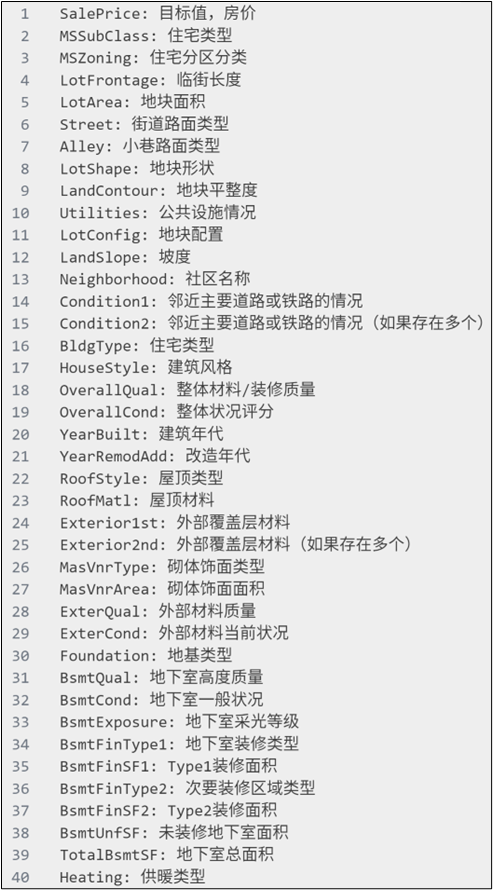
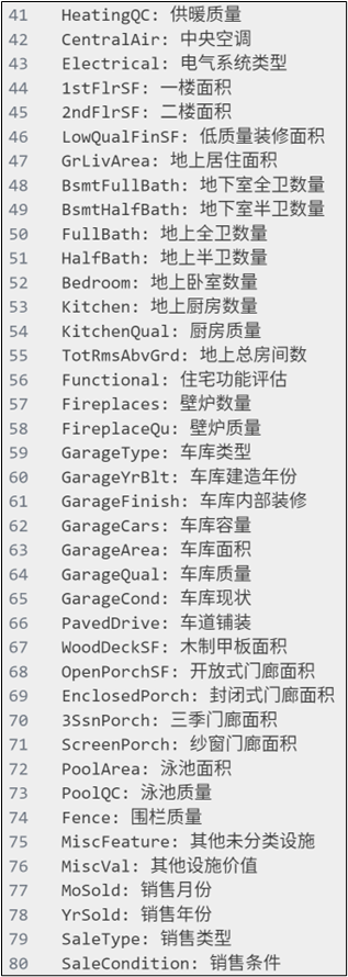
一、数据处理与特征工程Data Processing and Feature Engineering

首先读取数据并删除无关特征。

First, load the dataset and remove irrelevant features.

python 复制代码

data = pd.read_csv("../data/house_prices.csv")
data.drop(["Id"], axis=1, inplace=True)

其中 Id 对预测没有贡献，因此直接删除。

The Id column does not contribute to prediction and is removed.

目标变量是房价 SalePrice。

The target variable is SalePrice.

接下来划分特征与目标变量。

Next, split features and target variable.

python 复制代码

X = data.drop("SalePrice", axis=1)
y = data["SalePrice"]

然后划分训练集和测试集。

Then split the dataset into training and testing sets.

python 复制代码

x_train, x_test, y_train, y_test = train_test_split(
    X, y, test_size=0.2, random_state=42
)

固定随机种子可以保证实验结果可复现。

Setting a random seed ensures reproducibility.

对于表格数据，需要区分数值特征和类别特征。

For tabular data, numerical and categorical features must be separated.

python 复制代码

numerical_features = X.select_dtypes(include=['int64','float64']).columns
categorical_features = X.select_dtypes(include=['object','string']).columns

这是后续特征处理的基础。

This is the foundation for feature processing.

数值特征使用均值填充并进行标准化。

Numerical features are imputed with mean and standardized.

python 复制代码

numerical_transformer = Pipeline([
    ("fillna", SimpleImputer(strategy="mean")),
    ("std", StandardScaler()),
])

标准化可以加快模型训练收敛。

Standardization helps speed up convergence.

类别特征使用填充加 One-Hot 编码。

Categorical features are processed with imputation and One-Hot encoding.

python 复制代码

categorical_transformer = Pipeline([
    ('fillna', SimpleImputer(strategy='constant', fill_value='NaN')),
    ('onehot', OneHotEncoder(handle_unknown='ignore'))
])

忽略未知类别可以避免预测时报错。

Ignoring unknown categories prevents inference errors.

使用 ColumnTransformer 统一处理不同类型特征。

Use ColumnTransformer to combine different feature transformations.

python 复制代码

    # 列转换器
    column_transformer = ColumnTransformer([
        ('numerical', numerical_transformer, numerical_features),
        ('categorical', categorical_transformer, categorical_features)
    ])

随后对数据进行转换并转为张量格式。

Then transform the data and convert it to tensors.

python 复制代码

x_train = column_transformer.fit_transform(x_train).toarray()
x_test = column_transformer.transform(x_test).toarray()

这里将稀疏矩阵转为稠密矩阵以适配 PyTorch。

Sparse matrices are converted to dense format for PyTorch.

对目标值进行 log 变换是一个关键优化。

Applying log transformation to the target is a key optimization.

python 复制代码

y_train = torch.log(torch.clamp(torch.tensor(y_train.values).float(), 1, float('inf')))
y_test = torch.log(torch.clamp(torch.tensor(y_test.values).float(), 1, float('inf')))

这样可以缓解房价的长尾分布问题并提高稳定性。

This reduces long-tail distribution and improves training stability.

二、模型训练与结果分析Model Training and Evaluation

将数据封装为 Dataset 并使用 DataLoader。

Wrap the data into Dataset and use DataLoader.

python 复制代码

train_dataset = TensorDataset(torch.tensor(x_train).float(), y_train.view(-1,1))
train_loader = DataLoader(train_dataset, batch_size=64, shuffle=True)

这样可以实现 mini-batch 训练。

This enables mini-batch training.

模型采用简单的多层感知机结构。

The model is a simple multilayer perceptron.

python 复制代码

model = nn.Sequential(
    nn.Linear(input_features, 128),
    nn.BatchNorm1d(128),
    nn.ReLU(),
    nn.Dropout(0.2),
    nn.Linear(128, 1),
)

BatchNorm 和 Dropout 有助于提升泛化能力。

BatchNorm and Dropout improve generalization.

权重初始化采用 Kaiming 方法。

Weights are initialized using Kaiming initialization.

python 复制代码

def init_weights(layer):
    if isinstance(layer, nn.Linear):
        nn.init.kaiming_normal_(layer.weight)
        nn.init.zeros_(layer.bias)

优化器使用 Adam，损失函数使用 MSE。

The optimizer is Adam and the loss function is MSE.

python 复制代码

optimizer = optim.Adam(model.parameters(), lr=0.001)
mse_loss = nn.MSELoss()

训练过程遵循标准深度学习流程。

The training loop follows standard deep learning procedure.

python 复制代码

for epoch in range(epochs):
    model.train()
    for X, target in train_loader:
        optimizer.zero_grad()
        output = model(X)
        loss = mse_loss(output, target)
        loss.backward()
        optimizer.step()

包括前向传播、反向传播和参数更新。

It includes forward pass, backpropagation, and parameter updates.

验证阶段关闭梯度计算以提升效率。

Disable gradients during validation for efficiency.

python 复制代码

model.eval()
with torch.no_grad():
    for X, y in test_loader:
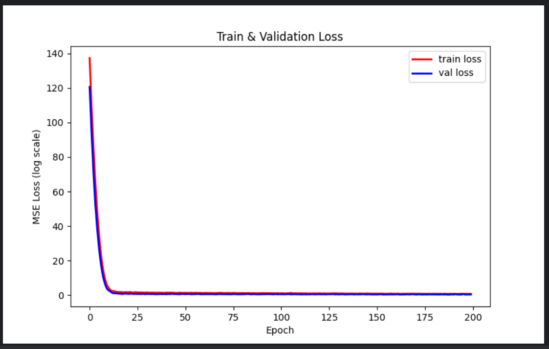
        output = model(X)

最后绘制训练与验证损失曲线。

Finally, plot training and validation loss curves.

python 复制代码

plt.plot(train_loss_list, label='train loss')
plt.plot(val_loss_list, label='val loss')
plt.legend()
plt.show()

三、网络结构设计 Network Architecture Design

模型采用一个简单的多层感知机（MLP）结构。

The model uses a simple Multilayer Perceptron (MLP).

python 复制代码

model = nn.Sequential(
    nn.Linear(input_features, 128),
    nn.BatchNorm1d(128),
    nn.ReLU(),
    nn.Dropout(0.2),
    nn.Linear(128, 1),
)

该结构由输入层、隐藏层和输出层组成。

The architecture consists of an input layer, hidden layer, and output layer.

第一层线性层将高维特征映射到 128 维隐空间。

The first linear layer maps high-dimensional input features into a 128-dimensional hidden space.

这一过程本质上是在学习特征之间的线性组合关系。

This step learns linear combinations of input features.

BatchNorm 层用于对隐藏层输出进行标准化。

BatchNorm normalizes the hidden layer activations.

它可以减少内部协变量偏移，从而加快模型收敛。

It reduces internal covariate shift and accelerates convergence.

ReLU 作为激活函数引入非线性能力。

ReLU introduces non-linearity into the model.

它的表达形式为：

Its formulation is:

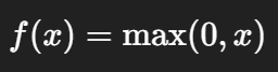
相比 sigmoid，ReLU 能有效缓解梯度消失问题。

Compared to sigmoid, ReLU alleviates the vanishing gradient problem.

Dropout 用于防止过拟合。

Dropout is used to prevent overfitting.

在训练过程中，它会随机丢弃一部分神经元：

During training, it randomly drops some neurons:

这相当于训练多个子网络的集成效果。

This acts like training an ensemble of subnetworks.

最后一层线性层输出一个标量，用于回归预测。

The final linear layer outputs a single value for regression.

由于目标值经过了 log 变换，因此模型输出的是对数空间的预测值。

Since the target is log-transformed, the model predicts values in log space.

相比树模型，MLP 更依赖特征缩放与分布处理，因此前面的标准化和 log 变换至关重要。

Compared to tree-based models, MLP relies more on feature scaling and distribution, making preprocessing crucial.

完整代码

python 复制代码

import torch
import pandas as pd
import torch.nn as nn
import matplotlib.pyplot as plt
from sklearn.model_selection import train_test_split
from sklearn.pipeline import Pipeline
from sklearn.impute import SimpleImputer  # 处理缺失值
from sklearn.compose import ColumnTransformer
from sklearn.preprocessing import StandardScaler, OneHotEncoder
from torch.utils.data import TensorDataset, DataLoader
import torch.optim as optim

def create_dataset():
    """构造数据集"""
    # 读取数据
    data = pd.read_csv("../data/house_prices.csv")
    # 去除无关特征
    data.drop(["Id"], axis=1, inplace=True)

    # 划分特征和目标
    X = data.drop("SalePrice", axis=1)
    y = data["SalePrice"]

    # 划分训练和测试集
    x_train, x_test, y_train, y_test = train_test_split(
        X, y, test_size=0.2, random_state=42
    )

    # 特征类型划分
    numerical_features = X.select_dtypes(include=['int64','float64']).columns
    categorical_features = X.select_dtypes(include=['object','string']).columns

    # 数值型特征 pipeline
    numerical_transformer = Pipeline([
        ("fillna", SimpleImputer(strategy="mean")),
        ("std", StandardScaler()),
    ])

    # 类别型特征 pipeline
    categorical_transformer = Pipeline([
        ('fillna', SimpleImputer(strategy='constant', fill_value='NaN')),
        ('onehot', OneHotEncoder(handle_unknown='ignore', sparse_output=True))
    ])

    # 列转换器
    column_transformer = ColumnTransformer([
        ('numerical', numerical_transformer, numerical_features),
        ('categorical', categorical_transformer, categorical_features)
    ])

    # 特征转换
    x_train = column_transformer.fit_transform(x_train).toarray()
    x_test = column_transformer.transform(x_test).toarray()

    # 对目标做 log 处理，保证训练稳定
    y_train = torch.log(torch.clamp(torch.tensor(y_train.values).float(), 1, float('inf')))
    y_test = torch.log(torch.clamp(torch.tensor(y_test.values).float(), 1, float('inf')))

    # 构建 dataset
    train_dataset = TensorDataset(torch.tensor(x_train).float(), y_train.view(-1,1))
    test_dataset = TensorDataset(torch.tensor(x_test).float(), y_test.view(-1,1))
    input_features = x_train.shape[1]

    return train_dataset, test_dataset, input_features

# 构建数据集
train_dataset, test_dataset, input_features = create_dataset()
print(len(train_dataset), len(test_dataset))

# 超参数
lr = 0.001
batch_size = 64
epochs = 200

# 数据加载器
train_loader = DataLoader(train_dataset, batch_size=batch_size, shuffle=True)
test_loader = DataLoader(test_dataset, batch_size=batch_size)

# 模型
model = nn.Sequential(
    nn.Linear(input_features, 128),
    nn.BatchNorm1d(128),
    nn.ReLU(),
    nn.Dropout(0.2),
    nn.Linear(128, 1),
)

# 初始化权重
def init_weights(layer):
    if isinstance(layer, nn.Linear):
        nn.init.kaiming_normal_(layer.weight)
        if layer.bias is not None:
            nn.init.zeros_(layer.bias)

model.apply(init_weights)

# 设备
device = torch.device("cuda:0" if torch.cuda.is_available() else "cpu")
model = model.to(device)

# 优化器
optimizer = optim.Adam(model.parameters(), lr=lr)

# 损失函数
mse_loss = nn.MSELoss()
def log_rmse(input, target):
    input = torch.clamp(input, 1, float("inf"))
    target = torch.clamp(target, 1, float("inf"))
    return torch.sqrt(nn.functional.mse_loss(input, target))

# 保存 loss
train_loss_list = []
val_loss_list = []

for epoch in range(epochs):
    # ===== 训练 =====
    model.train()
    train_loss_total = 0
    for X, target in train_loader:
        X, target = X.to(device), target.to(device)

        optimizer.zero_grad()
        output = model(X)
        loss = mse_loss(output, target)
        loss.backward()
        optimizer.step()

        train_loss_total += loss.item() * X.shape[0]

    this_train_loss = train_loss_total / len(train_dataset)
    train_loss_list.append(this_train_loss)

    # ===== 验证 =====
    model.eval()
    val_loss_total = 0
    with torch.no_grad():
        for X, y in test_loader:
            X, y = X.to(device), y.to(device)
            output = model(X)
            loss = mse_loss(output, y)
            val_loss_total += loss.item() * X.shape[0]

    this_val_loss = val_loss_total / len(test_dataset)
    val_loss_list.append(this_val_loss)

    print(f"Epoch {epoch+1}, train loss: {this_train_loss:.4f}, val loss: {this_val_loss:.4f}")

# ===== 绘制 loss 曲线 =====
plt.figure(figsize=(8,5))
plt.plot(train_loss_list, 'r-', label='train loss', linewidth=2)
plt.plot(val_loss_list, 'b-', label='val loss', linewidth=2)
plt.legend()
plt.xlabel("Epoch")
plt.ylabel("MSE Loss (log scale)")
plt.title("Train & Validation Loss")
plt.show()