一、写在前面
在跨物种单细胞研究中,如何消除物种间的进化差异并实现细胞类型的精确比对,是单细胞转录组(scRNA-seq)分析中的难点。针对南极鱼(Trematomus bernacchii, TB)与尼罗罗非鱼(Oreochromis niloticus, ON)的脑组织数据,本教程展示了从 Cell Ranger 原始流程启动,到利用Diamond进行跨物种同源基因预测,并最终通过CCA (Canonical Correlation Analysis) 算法实现多物种数据集整合的完整管线。
在分析过程中,我们不仅引入了Scrublet算法来精准拦截模拟双细胞,还针对非模式物种研究中常见的基因注释不全问题,演示了如何通过解析GFF3注释文件自定义基因名映射表。通过对比Harmony与CCA在跨物种整合上的表现,让我们在复杂进化背景下,从数万个细胞中抽丝剥茧,定位保守的神经元亚群及其差异表达特征。
如果需要单细胞数据分析 指导 、生信热点全文复现 、自测数据个性化分析 辅导 、常态化实验学习 ,欢迎联系**Biomamba_zhushou**。
二、实操流程
1.准备工作
1.1 安装cellranger
下载解压安装包
cd /storage/public/yongpeng/work/cellranger

wget -O cellranger-10.0.0.tar.gz "https://cf.10xgenomics.com/releases/cell-exp/cellranger-10.0.0.tar.gz?Expires=1775781670&Key-Pair-Id=APKAI7S6A5RYOXBWRPDA&Signature=Z51eZif2whpR7Rmp-It1rTPG-P2Z9UOHm-MgqSjds~AJs3cuf98cL0a1oLI8neaeZom72Sr9PQQv8KR3bbWSz1qpNuCMbkgtlG0l7SUC64q7ZTAR8oBmMd~lyfY5961Ba9dnPPtr-JS94SCKHnaAtzv6LfDoWUIu2HZkTi8~eWufI8MjxZCWaMldoQCOkxUBtTwnTUKR-EZjSKCX2ZAt7Ip3-dWcVb2QayDesuRbP~MrN7akrqrCY8~Lfcuv2H7rmc3~yeuklrg0A~DekYqjXny--bouLBVnTzUhyTUx8wZgjgVPBralpU~RuoJkS6Yaklu1nSGpcTK71ozwjhl61A__"

tar -zxvf /storage/public/yongpeng/work/cellranger/cellranger-7.1.0.tar.gz
配置软件路径以及检查是否安装成功
配置软件路径方便后续直接使用cellranger
echo 'export PATH=/storage/public/yongpeng/work/cellranger/cellranger-7.1.0:$PATH' >> ~/.bashrc

source .bashrc
尝试使用cellranger看是否安装成功
cellrangercellranger cellranger-7.1.0 Process 10x Genomics Gene Expression, Feature Barcode, and Immune Profiling data
USAGE: cellranger
OPTIONS: -h, --help Print help information -V, --version Print version information
SUBCOMMANDS: count Count gene expression (targeted or whole-transcriptome) and/or feature barcode reads from a single sample and GEM well multi Analyze multiplexed data or combined gene expression/immune profiling/feature barcode data multi-template Output a multi config CSV template vdj Assembles single-cell VDJ receptor sequences from 10x Immune Profiling libraries aggr Aggregate data from multiple Cell Ranger runs reanalyze Re-run secondary analysis (dimensionality reduction, clustering, etc) targeted-compare Analyze targeted enrichment performance by comparing a targeted sample to its cognate parent WTA sample (used as input for targeted gene expression) targeted-depth Estimate targeted read depth values (mean reads per cell) for a specified input parent WTA sample and a target panel CSV file mkvdjref Prepare a reference for use with CellRanger VDJ mkfastq Run Illumina demultiplexer on sample sheets that contain 10x-specific sample index sets testrun Execute the 'count' pipeline on a small test dataset mat2csv Convert a gene count matrix to CSV format mkref Prepare a reference for use with 10x analysis software. Requires a GTF and FASTA mkgtf Filter a GTF file by attribute prior to creating a 10x reference upload Upload analysis logs to 10x Genomics support sitecheck Collect linux system configuration information help Print this message or the help of the given subcommand(s)
表明安装成功
1.2 准备单细胞测序数据
ls /storage/public/yongpeng/work/cellranger/ONRNAT2RNA_S1_L001_R1_001.fastq.gz T2RNA_S2_L001_R2_001.fastq.gz T2RNA_S4_L001_R1_001.fastq.gz T2RNA_S1_L001_R2_001.fastq.gz T2RNA_S3_L001_R1_001.fastq.gz T2RNA_S4_L001_R2_001.fastq.gz T2RNA_S2_L001_R1_001.fastq.gz T2RNA_S3_L001_R2_001.fastq.gz
ls /storage/public/yongpeng/work/cellranger/TBRNATBRNA_S1_L001_R1_001.fastq.gz TBRNA_S2_L001_R2_001.fastq.gz TBRNA_S4_L001_R1_001.fastq.gz TBRNA_S1_L001_R2_001.fastq.gz TBRNA_S3_L001_R1_001.fastq.gz TBRNA_S4_L001_R2_001.fastq.gz TBRNA_S2_L001_R1_001.fastq.gz TBRNA_S3_L001_R2_001.fastq.gz
1.3 下载基因组文件和注释文件
ON数据(Oreochromis_niloticus)
wget https://ftp.ensembl.org/pub/release-115/fasta/oreochromis_niloticus/dna/Oreochromis_niloticus.O_niloticus_UMD_NMBU.dna.toplevel.fa.gz
wget https://ftp.ensembl.org/pub/release-115/gtf/oreochromis_niloticus/Oreochromis_niloticus.O_niloticus_UMD_NMBU.115.gtf.gz
TB数据(Trematomus_bernacchii)此基因组文件和注释文件是实验室组装制作
1.4 运行cellranger
nohup cellranger mkref \
    --genome=Oni_genome_rna \
    --fasta=Oreochromis_niloticus.O_niloticus_UMD_NMBU.dna.toplevel.fa \
    --genes=Oreochromis_niloticus.O_niloticus_UMD_NMBU.111.gtf &

nohup /cellranger count \
--id=ON_cellranger\
--transcriptome=/storage/public/yongpeng/work/cellranger/Oni_genome_rna \
--fastqs=/storage/public/yongpeng/work/cellranger/ONRNA \
--sample=T2RNA \
--create-bam=true > $s.log 2>&1 &

nohup cellranger mkref \
    --genome=TB_genome_rna \
    --fasta=Trematomus_bernacchii.dna.fa \
    --genes=Trematomus_bernacchii.gtf &

nohup cellranger count \
--id=TB_cellranger \
--transcriptome=/storage/public/yongpeng/work/cellranger/TB_genome_rna \
--fastqs=/storage/public/yongpeng/work/cellranger/T2RNA \
--sample=TBRNA \
--create-bam=true > $s.log 2>&1 &

ls /storage/public/yongpeng/work/cellranger/ON_cellranger
cmdline _finalstate _log _perf _sitecheck _timestamp _versions extras _invocation _mrosource _perf._truncated _tags _uuid _filelist _jobmode outs SC_RNA_COUNTER_CS ON.mri.tgz _vdrkill 检查目录是否完整
若要合并不同物种的数据,需要先统一基因名,这里通过寻找同源基因来达成目的,由于ON物种基因研究较为全面因此把TB基因转换成ON对应的同源基因。
1.5 注释同源基因
准备两个物种的蛋白序列文件TB是实验室提供,ON需要从ENSEMBL下载
cd /home/yongpeng/work/blast/diamond

wget https://ftp.ensembl.org/pub/release-115/fasta/oreochromis_niloticus/pep/Oreochromis_niloticus.O_niloticus_UMD_NMBU.pep.all.fa.gz
Eggnog的比对结果相比于diamond更准确,但是由于运行时间过长,这里仅使用diamond作为示例
nohup diamond makedb --in Oreochromis_niloticus.O_niloticus_UMD_NMBU.pep.all.fa.gz --db ON_diamond &

nohup diamond blastp -q Trematomus_bernacchii.pep.faa --db ON_diamond --out /home/yongpeng/work/blast/diamond/TB_ON -p 4 &
提取出基因对应表(每个对应关系只保留匹配度最高,匹配度低于80%则删除)保存为TB_TO_ON.xlsx
2.单细胞测序数据质控
使用jupyter平台连接服务器进行R语言和python分析
conda activate jupyter
jupyter notebook --no-browser
2.1 使用python标注 双细胞
这里使用Scrublet方法,基于模拟双细胞+k近邻分类的算法,用于检测单细胞 RNA 测序数据中的技术性双细胞。
import numpy as np
import pandas as pd
import scanpy as sc
读取原始测序文件
ON_brain <- "/storage/public/yongpeng/work/cellranger/ON_cellranger/outs/ON_filtered_feature_bc_matrix.h5"
TB_brain <- "/storage/public/yongpeng/work/cellranger/TB_cellranger/outs/TB_filtered_feature_bc_matrix.h5"

adata_ON = sc.read_10x_mtx(ON_brain,var_names='gene_ids',cache=True)
adata_ON
AnnData object with n_obs × n_vars = 12947 × 32125
var: 'gene_symbols', 'feature_types'
adata_TB = sc.read_10x_mtx(TB_brain,var_names='gene_ids',cache=True)检测并标记出单细胞数据中可能由技术误差产生的双细胞
sc.pp.scrublet(adata_ON)
sc.pp.scrublet(adata_TB)

sc.pl.scrublet_score_distribution(adata_ON)
sc.pl.scrublet_score_distribution(adata_TB)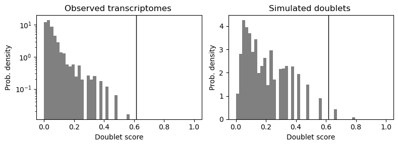
adata_ON 样本的上样浓度较低,预期双细胞率低,因此用更低的阈值(0.16)可能仍能保持较低假阳性;而 adata_TB 样本上样浓度高,双细胞率高,需要更高阈值(0.2)来平衡假阳性和假阴性。
sc.pp.scrublet(adata_ON,threshold=0.16)
sc.pp.scrublet(adata_CH,threshold=0.2)
对双细胞进行标记方便后续更具标记删除双细胞
adata_TB = adata_TB[~adata_TB.obs['predicted_doublet']]
adata_ON = adata_ON[~adata_ON.obs['predicted_doublet']]

sc.pp.filter_cells(adata_TB, min_genes=100)
sc.pp.filter_genes(adata_TB, min_cells=3)
sc.pp.filter_cells(adata_ON, min_genes=100)
sc.pp.filter_genes(adata_ON, min_cells=3)
讲标记好的文件保存用以后续筛选
adata_TB_bc_df = pd.DataFrame(adata_TB.obs.index,columns=['barcode'])
adata_TB_bc_df.to_csv('./adata_TB_barcodes.csv',index=False)

adata_TB_bc_df = pd.DataFrame(adata_TB.obs.index,columns=['barcode'])
adata_TB_bc_df.to_csv('./adata_ON_barcodes.csv',index=False)
得到双细胞标注文件
这里开始转换成R语言
除了去除双细胞外,还要再这一步替换TB中原基因为ON的同源基因以便后续分析
library(dplyr)
library(Seurat)
library(patchwork)
library(ggplot2)
library(data.table)
library("Matrix")
Attaching package: 'dplyr'
The following objects are masked from 'package:stats':
filter, lag
The following objects are masked from 'package:base':
intersect, setdiff, setequal, union
Warning message:
"package 'Seurat' was built under R version 4.3.3"
Loading required package: SeuratObject
Warning message:
"package 'SeuratObject' was built under R version 4.3.3"
Loading required package: sp
Attaching package: 'SeuratObject'
The following objects are masked from 'package:base':
intersect, t
Attaching package: 'data.table'
The following objects are masked from 'package:dplyr':
between, first, last
ON_brain <- "/storage/public/yongpeng/work/cellranger/ON_cellranger/outs/ON_filtered_feature_bc_matrix.h5"
TB_brain <- "/storage/public/yongpeng/work/cellranger/TB_cellranger/outs/TB_filtered_feature_bc_matrix.h5"

names(ON_dir) <- c("ON_brain")
names(TB_dir) <- c("TB_brain")

ct <- Read10X_h5(ON_dir, use.names = F)
if(inherits(ct, "list")){
    ct <- ct$`Gene Expression`
}
colnames(ct) <- paste(names(ON_dir), colnames(ct), sep = "_")
TB_ct <- dat_combined_Ti <- dsCombineDGE(sceList)

ct <- Read10X_h5(TB_dir, use.names = F)
if(inherits(ct, "list")){
    ct <- ct$`Gene Expression`
}
colnames(ct) <- paste(names(TB_dir), colnames(ct), sep = "_")
TB_ct <- ct
提前准备后续跨物种整合做准备
注释TB基因为ON同源基因
oldnames <- data.frame(TB_ID = rownames(TB_ct))
writeLines(oldnames, "/storage/public/yongpeng/work/H5/oldnames.txt")
library(readxl)
library(openxlsx)
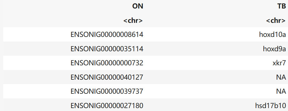
TB_to_ON <- read_excel("TB_to_ON.xlsx")
names(TB_to_ON) <- c("ON", "TB")
head(TB_to_ON)A tibble: 6 × 2
newname <- merge(oldnames, TB_to_ON, by = "TB", all.x = TRUE, sort = FALSE)
# 用 match 确保顺序
newname <- newname[match(oldnames$TB, newname$TB), ]

rownames(TB_ct) <- newname

saveRDS(TB_ct,file='/storage/public/yongpeng/work/H5/H5.ON_brain.rds')
saveRDS(TB_ct,file='/storage/public/yongpeng/work/HE/H5.TB_brain.rds')

sc_ON <- CreateSeuratObject(counts = ON_ct,min.cells = 3,min.features = 200)
sc_Tb <- CreateSeuratObject(counts = TB_ct,min.cells = 3,min.features = 200)
#需要根据自己的数据调整参数

saveRDS(sc_ON,file='/storage/public/yongpeng/work/cellranger/ON_brain.rds')
saveRDS(sc_Tb,file='/storage/public/yongpeng/work/cellranger/TB_brain.rds')

sc_ON$orig.ident <- "ON"
sc_Tb$orig.ident <- "TB"

ON_bc <- read.csv('adata_ON_barcodes.csv')
TB_bc <- read.csv('adata_TB_barcodes.csv')

barcodes_to_keep <- ON_bc$barcode
sc_ON$barcode <- colnames(sc_ON)
ON_filtered <- subset(sc_ON,subset = ON_bc$barcode %in% barcodes_to_keep)

barcodes_to_keep <- TB_bc$barcode
sc_Tb$barcode <- colnames(sc_Tb)
TB_filtered <- subset(sc_Tb,subset = sc_Tb$barcode %in% barcodes_to_keep)

saveRDS(TB_filtered,file = "TB.doublefiltered.rds")
saveRDS(ON_filtered,file = "ON.doublefiltered.rds")
至此得到去除双细胞的seurat文件
2.2 QC质控
ON数据质控
# 修改active.ident
new_identity <- rep("ON-brain", length(ON_filtered@active.ident))
new_identity <- factor(new_identity)
ON_filtered@active.ident <- new_identity
ON_filtered@active.ident <- factor(ON_filtered@active.ident)
names(ON_filtered@active.ident) <- colnames(ON_filtered)
print(dim(ON_filtered))
mt.genes <- rownames(ON_filtered)[grepl("mt-", rownames(ON_filtered))]
ON_filtered[["percent.mt"]] <- PercentageFeatureSet(ON_filtered, features = intersect(rownames(ON_filtered),mt.genes))
1 25275 8811
options(repr.plot.width = 10,repr.plot.height = 5)
VlnPlot(ON_filtered, features = c("nFeature_RNA", "nCount_RNA", "percent.mt"), ncol = 3,pt.size = 0)
FeatureScatter(ON_filtered, feature1 = "nCount_RNA", feature2 = "percent.mt", pt.size = 0.5)
FeatureScatter(ON_filtered, feature1 = "nCount_RNA", feature2 = "nFeature_RNA", pt.size = 0.5)
Warning message:
"Default search for "data" layer in "RNA" assay yielded no results; utilizing "counts" layer instead."
Warning message:
"The `slot` argument of `FetchData()` is deprecated as of SeuratObject 5.0.0.
ℹ Please use the `layer` argument instead.
ℹ The deprecated feature was likely used in the Seurat package.
Please report the issue at <https://github.com/satijalab/seurat/issues\>."
Warning message:
"`PackageCheck()` was deprecated in SeuratObject 5.0.0.
ℹ Please use `rlang::check_installed()` instead.
ℹ The deprecated feature was likely used in the Seurat package.
Please report the issue at <https://github.com/satijalab/seurat/issues\>."
qc_metrics <- list(
Brain.nFeature = quantile(ON_filtered$nFeature_RNA, probs = c(0.01, 0.99)),
Brain.percent.mt = median(ON_filtered$percent.mt) + 3 * mad(ON_filtered$percent.mt),
ON.nFeature = quantile(ON_filtered$nFeature_RNA, probs = c(0.01, 0.99)),
ON.percent.mt = median(ON_filtered$percent.mt) + 3 * mad(ON_filtered$percent.mt)
)
qc_metrics
#进行筛选
qc_filter_report <- function(seurat_obj, min_features = 300, mt_thresholds = c(30, 25, 20, 15, 10, 5)) {
total_cells <- ncol(seurat_obj)
results <- data.frame(
percent_mt_threshold = numeric(),
retained_cells = integer(),
retained_percent = numeric()
)
for (threshold in mt_thresholds) {
filtered <- subset(seurat_obj, subset = nFeature_RNA > min_features & percent.mt < threshold)
retained <- ncol(filtered)
percent_retained <- round((retained / total_cells) * 100, 2)
results <- rbind(results, data.frame(
percent_mt_threshold = threshold,
retained_cells = retained,
retained_percent = percent_retained
))
}
return(results)
}
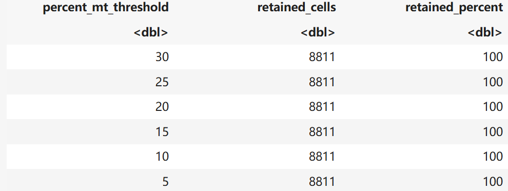
qc_filter_report(ON_filtered)
ON_filtered <- subset(ON_filtered, subset = nFeature_RNA > 300 & percent.mt < 5)$Brain.nFeature 1%:513 99%:4852.3
$Brain.percent.mt 0.724381513770556
$ON.nFeature 1%:513 99%:4852.3
$ON.percent.mt 0.724381513770556
A data.frame: 6 × 3
saveRDS(ON_filtered,file = "ON.dc.qc.rds")TB数据质控同上
# 修改active.ident
new_identity <- rep("TB-brain", length(TB_filtered@active.ident))
new_identity <- factor(new_identity)
TB_filtered@active.ident <- new_identity
TB_filtered@active.ident <- factor(TB_filtered@active.ident)
names(TB_filtered@active.ident) <- colnames(TB_filtered)
print(dim(TB_filtered))
mt.genes <- rownames(TB_filtered)[grepl("mt-", rownames(TB_filtered))]
TB_filtered[["percent.mt"]] <- PercentageFeatureSet(TB_filtered, features = intersect(rownames(TB_filtered),mt.genes))
options(repr.plot.width = 10,repr.plot.height = 5)
VlnPlot(TB_filtered, features = c("nFeature_RNA", "nCount_RNA", "percent.mt"), ncol = 3,pt.size = 0)
FeatureScatter(TB_filtered, feature1 = "nCount_RNA", feature2 = "percent.mt", pt.size = 0.5)
FeatureScatter(TB_filtered, feature1 = "nCount_RNA", feature2 = "nFeature_RNA", pt.size = 0.5)
qc_metrics <- list(
Brain.nFeature = quantile(TB_filtered$nFeature_RNA, probs = c(0.01, 0.99)),
Brain.percent.mt = median(TB_filtered$percent.mt) + 3 * mad(TB_filtered$percent.mt),
TB.nFeature = quantile(TB_filtered$nFeature_RNA, probs = c(0.01, 0.99)),
TB.percent.mt = median(TB_filtered$percent.mt) + 3 * mad(TB_filtered$percent.mt)
)
qc_metrics
#进行筛选
qc_filter_report <- function(seurat_obj, min_features = 300, mt_thresholds = c(30, 25, 20, 15, 10, 5)) {
total_cells <- ncol(seurat_obj)
results <- data.frame(
percent_mt_threshold = numeric(),
retained_cells = integer(),
retained_percent = numeric()
)
for (threshold in mt_thresholds) {
filtered <- subset(seurat_obj, subset = nFeature_RNA > min_features & percent.mt < threshold)
retained <- ncol(filtered)
percent_retained <- round((retained / total_cells) * 100, 2)
results <- rbind(results, data.frame(
percent_mt_threshold = threshold,
retained_cells = retained,
retained_percent = percent_retained
))
}
return(results)
}
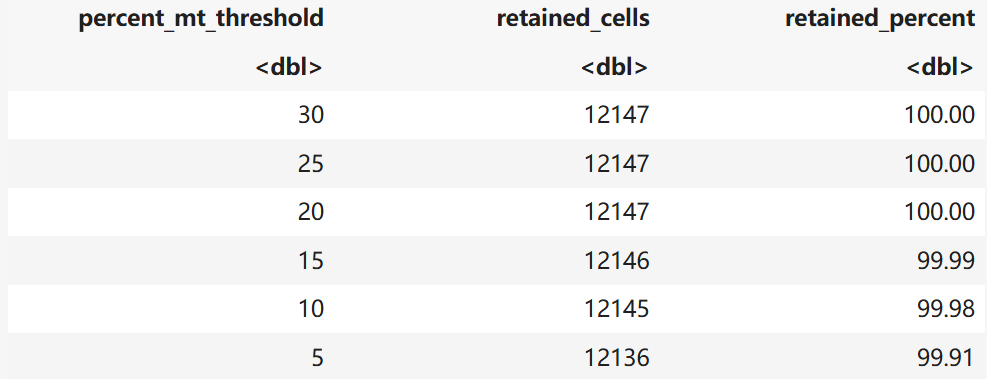
qc_filter_report(TB)
TB <- subset(TB, subset = nFeature_RNA > 300 & percent.mt < 5)
saveRDS(TB,file = "TB.dc.qc.rds")1 24803 12147
Warning message:
"Default search for "data" layer in "RNA" assay yielded no results; utilizing "counts" layer instead."
$Brain.nFeature 1%:448 99%:5770.54
$Brain.percent.mt 1.62767957625196
$TB.nFeature 1%:448 99%:5770.54
$TB.percent.mt 1.62767957625196
A data.frame: 6 × 3
3. CCA整合步骤
library(Seurat)
library(dplyr)
library(ggplot2)
library(tidyr)
library(patchwork)
library(Matrix)
library(harmony)
Attaching package: 'tidyr'
The following objects are masked from 'package:Matrix':
expand, pack, unpack
Loading required package: Rcpp
TB<- readRDS("TB.dc.qc.rds")
ON<- readRDS("ON.dc.qc.rds")

common_genes <- intersect(rownames(TB), rownames(ON))

sc_lc <- merge(TB,y = ON)

sc_lc
An object of class Seurat
35067 features across 20816 samples within 1 assay
Active assay: RNA (35067 features, 2000 variable features)
5 layers present: counts.tb, counts.SeuratProject, data.SeuratProject, scale.data.6.SeuratProject, scale.data.SeuratProject
head(common_genes)'ENSONIG00000008614''ENSONIG00000035114''ENSONIG00000000732'
'ENSONIG00000027180''ENSONIG00000016575''ENSONIG00000016573'
只保留ON和TB共有基因,特有基因不纳入跨物种比对范围
sc_filtered <- subset(sc_lc, features = common_genes)

sc_filtered <- sc_filtered[,sc_filtered$nFeature_RNA < 4000]
sc_filtered
An object of class Seurat
15774 features across 20170 samples within 1 assay
Active assay: RNA (15774 features, 1257 variable features)
5 layers present: counts.tb, counts.SeuratProject, data.SeuratProject, scale.data.6.SeuratProject, scale.data.SeuratProject
常规整合查看整体情况
sc_filtered <- sc_filtered %>%
      NormalizeData(verbose = F) %>%
      FindVariableFeatures(verbose = F) %>%
      ScaleData(verbose = F) %>%
      RunPCA(verbose = FALSE) %>%
      FindNeighbors(reduction = "pca", dims = 1:30,verbose = F) %>%
      FindClusters(resolution = c(0.1,0.2),cluster.name = c('unintegrated_clusters_0.1','unintegrated_clusters_0.2'),verbose = F) %>%
      RunUMAP(reduction = "pca", dims = 1:30, reduction.name = "umap.unintegrated", verbose = FALSE)
Warning message:
"The default method for RunUMAP has changed from calling Python UMAP via reticulate to the R-native UWOT using the cosine metric
To use Python UMAP via reticulate, set umap.method to 'umap-learn' and metric to 'correlation'
This message will be shown once per session"
options(repr.plot.width = 8, repr.plot.height = 8)
plot1 <- DimPlot(sc_filtered, reduction = "umap.unintegrated", label = T, group.by = "unintegrated_clusters_0.1") + NoLegend()
plot2 <- DimPlot(sc_filtered, reduction = "umap.unintegrated", label = T, group.by = "unintegrated_clusters_0.2") + NoLegend()
plot3 <- DimPlot(sc_filtered, reduction = "umap.unintegrated", label = T, group.by = "orig.ident") + NoLegend()
plot1 + plot2 + plot3  + plot_layout(nrow = 2)

sc_filtered <- RunHarmony(sc_filtered, group.by = "orig.ident")
Transposing data matrix
Initializing state using k-means centroids initialization
Harmony 1/10
Harmony 2/10
Harmony 3/10
Harmony 4/10
Harmony 5/10
Harmony converged after 5 iterations
Warning message:
"The `slot` argument of `GetAssayData()` is deprecated as of SeuratObject 5.0.0.
ℹ Please use the `layer` argument instead.
ℹ The deprecated feature was likely used in the Seurat package.
Please report the issue at <https://github.com/satijalab/seurat/issues\>."
sc_filtered <- IntegrateLayers(
  object = sc_filtered, method = HarmonyIntegration,
  orig.reduction = "pca", new.reduction = "harmony",
  verbose = FALSE
)
The `features` argument is ignored by `HarmonyIntegration`.
This message is displayed once per session.
sc_filtered <- sc_filtered %>%
  FindNeighbors(reduction = "harmony", dims = 1:30,verbose = F) %>%
  FindClusters(resolution = c(0.1,0.2),cluster.name = c('harmony_clusters_0.1','harmony_clusters_0.2'),verbose = F) %>%
  RunUMAP(reduction = "harmony", dims = 1:30,reduction.name = 'umap.harmony',verbose = FALSE)

options(repr.plot.width = 8, repr.plot.height = 8)
plot1 <- DimPlot(sc_filtered, reduction = "umap.harmony", label = T, group.by = "harmony_clusters_0.1") + NoLegend()
plot2 <- DimPlot(sc_filtered, reduction = "umap.harmony", label = T, group.by = "harmony_clusters_0.2") + NoLegend()
plot3 <- DimPlot(sc_filtered, reduction = "umap.harmony", label = T, group.by = "orig.ident") + NoLegend()
plot1 + plot2 + plot3 + plot_layout(nrow = 2)
使用CCA
brain.split <- SplitObject(sc_lc, split.by = "orig.ident")

brain.split
$TB
An object of class Seurat
24803 features across 12136 samples within 1 assay
Active assay: RNA (24803 features, 1186 variable features)
1 layer present: counts.tb
$T6
An object of class Seurat
25500 features across 8680 samples within 1 assay
Active assay: RNA (25500 features, 2000 variable features)
4 layers present: counts.SeuratProject, data.SeuratProject, scale.data.6.SeuratProject, scale.data.SeuratProject
brain.split <- lapply(brain.split, function(x) {
  x <- NormalizeData(x, verbose = FALSE)
  x <- FindVariableFeatures(x, selection.method = "vst", nfeatures = 2000)
  return(x)
})
# 选择跨数据集的共有高变基因
features <- SelectIntegrationFeatures(object.list = brain.split)
# 使用FindIntegrationAnchors函数识别锚点
anchors <- FindIntegrationAnchors(object.list = brain.split, anchor.features = features)
# 使用IntegrateData函数整合数据集
integrated_data <- IntegrateData(anchorset = anchors)
Finding variable features for layer counts.tb
Finding variable features for layer counts.SeuratProject
Scaling features for provided objects
Finding all pairwise anchors
Running CCA
Merging objects
Warning message:
"The `slot` argument of `SetAssayData()` is deprecated as of SeuratObject 5.0.0.
ℹ Please use the `layer` argument instead.
ℹ The deprecated feature was likely used in the Seurat package.
Please report the issue at <https://github.com/satijalab/seurat/issues\>."
Finding neighborhoods
Finding anchors
Found 15499 anchors
Filtering anchors
Retained 6187 anchors
Finding neighborhoods
Finding anchors
Found 15499 anchors
Filtering anchors
Retained 6187 anchors
Merging dataset 2 into 1
Extracting anchors for merged samples
Finding integration vectors
Warning message:
"Different features in new layer data than already exists for scale.data"
Finding integration vector weights
Integrating data
Warning message:
"Layer counts isn't present in the assay object; returning NULL"
integrated_data <-ScaleData(integrated_data ,verbose = F)

integrated_data

integrated_data <- RunPCA(integrated_data, verbose = FALSE)
integrated_data <- FindNeighbors(integrated_data, dims = 1:30, reduction = "pca",verbose = F)
integrated_data <-FindClusters(integrated_data, resolution = c(0.1,0.2,0.4),cluster.name = c('CCA_clusters_0.1','CCA_clusters_0.2','CCA_clusters_0.4'),verbose = F)
integrated_data <- RunUMAP(integrated_data, reduction = "pca", dims = 1:30,
                       reduction.name = "umap.unintegrated", verbose = FALSE)

options(repr.plot.width = 8, repr.plot.height = 8)
plot1 <- DimPlot(integrated_data, reduction = "umap.unintegrated", label = T, group.by = "CCA_clusters_0.1") + NoLegend()
plot2 <- DimPlot(integrated_data, reduction = "umap.unintegrated", label = T, group.by = "CCA_clusters_0.2") + NoLegend()
plot3 <- DimPlot(integrated_data, reduction = "umap.unintegrated", label = T, group.by = "orig.ident") + NoLegend()
plot1 + plot2 + plot3  + plot_layout(nrow = 2)

saveRDS(integrated_data,file="brain.CCATBON.rds")

options(repr.plot.width = 10, repr.plot.height = 5)
DimPlot(integrated_data,  label = T,repel = T,split.by = "orig.ident", group.by = "CCA_clusters_0.1")

options(repr.plot.width = 10, repr.plot.height = 5)
DimPlot(integrated_data,  label = T,repel = T,split.by = "orig.ident", group.by = "CCA_clusters_0.2")
CCA聚类情况相比于Harmony较好
4.进行细胞簇注释
biomart可以用于注释基因名对应表,但是由于版本更新问题,时长会遗漏部分基因,相比之下直接从最新gff3文件中提取基因名对应表更全
下载gff3注释文件到本地
cd /storage/public/yongpeng/work/cellranger

wget https://ftp.ensembl.org/pub/release-115/gff3/oreochromis_niloticus/Oreochromis_niloticus.O_niloticus_UMD_NMBU.111.gff3.gz
从gff3注释文件中提取和基因名对应表ON.EN_to_name.xlsx
# 输入文件路径
input_file="/storage/public/yongpeng/work/cellranger/Oreochromis_niloticus.O_niloticus_UMD_NMBU.111.gff3"
# 输出文件路径
output_file="ON.EN_to_name.txt"
# 使用awk提取基因Ensembl号和基因名
awk -F'\t' '{
    if ($3 == "gene") {
        # 提取属性字段
        attributes = $9
        # 初始化Ensembl号和基因名
        ensembl_id = ""
        gene_name = ""
        # 分割属性字段
        n = split(attributes, arr, ";")
        for (i = 1; i <= n; i++) {
            # 提取Ensembl号(通常是ID字段)
            if (arr[i] ~ /ID=/) {
                ensembl_id = arr[i]
                sub(/ID=/, "", ensembl_id)
            }
            # 提取基因名
            if (arr[i] ~ /Name=/) {
                gene_name = arr[i]
                sub(/Name=/, "", gene_name)
            }
        }
        if (ensembl_id != "" && gene_name != "") {
            print ensembl_id "\t" gene_name
        }
    }
}' "$input_file" > "$output_file"
echo "基因Ensembl号和基因名的对应表已保存到 $output_file"
基因Ensembl号和基因名的对应表已保存到 ON.EN_to_name.txt
head ON.EN_to_name.xlsxgene:ENSONIG00000015575 ctsd gene:ENSONIG00000015584 sirt3 gene:ENSONIG00000030102 DRD4 gene:ENSONIG00000015587 psmd13 gene:ENSONIG00000015598 csnk2a2a gene:ENSONIG00000015601 MATCAP1 gene:ENSONIG00000034066 zgc:194679 gene:ENSONIG00000007022 ppip5k1a gene:ENSONIG00000029455 map1aa gene:ENSONIG00000007015 tp53bp1
library(Seurat)
library(dplyr)
library(ggplot2)
library(tidyr)
library(patchwork)
library(Matrix)
library(harmony)
修改基因id用于后续的maker注释
#寻找maker用于注释
integrated_data<- readRDS("brain.CCATBON.rds")
Idents(integrated_data) = "CCA_clusters_0.1"
mak <- FindAllMarkers(integrated_data, only.pos = TRUE,logfc.threshold = 0.5)
#修改基因id便于后续的maker注释
library(readxl)
library(openxlsx)
library(dplyr)
tilapia_id_name <- read.table("ON.EN_to_name.xlsx", sep = "\t")
colnames(tilapia_id_name) <- c("Gene.stable.ID", "Gene.name")
write.xlsx(tilapia_id_name, "ON.EN_to_name.xlsx")
tilapia_id_name$Gene.stable.ID <- gsub("^gene:", "", tilapia_id_name$Gene.stable.ID, ignore.case = TRUE)
tilapia_id_name <- tilapia_id_name %>%
distinct(Gene.stable.ID, .keep_all = TRUE)
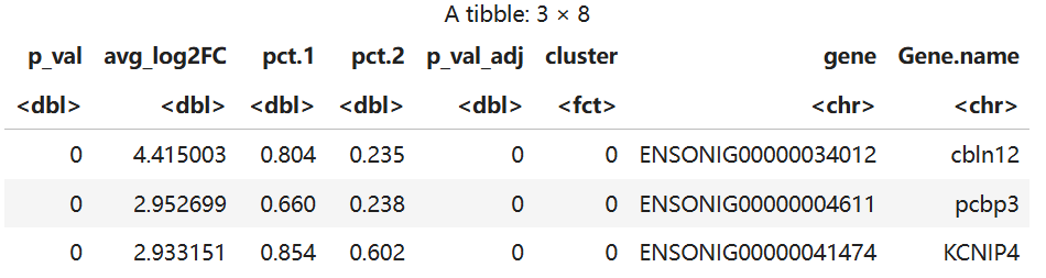
mak <- mak %>%
filter(p_val_adj <0.01 & pct.1 > 0.1) %>%
group_by(gene) %>%
left_join(tilapia_id_name[,c(1,2)],by = c("gene"="Gene.stable.ID"),multiple = "first") %>%
ungroup
head(mak,3)
write.table(mak,'TBONCCA.MAK',sep = '\t',row.names = F)Calculating cluster 0
Warning message in mean.fxn(objectfeatures, cells.1, drop = FALSE):
"NaNs produced"
Warning message in mean.fxn(objectfeatures, cells.2, drop = FALSE):
"NaNs produced"
Warning message:
"`PackageCheck()` was deprecated in SeuratObject 5.0.0.
ℹ Please use `rlang::check_installed()` instead.
ℹ The deprecated feature was likely used in the Seurat package.
Please report the issue at <https://github.com/satijalab/seurat/issues\>."
Calculating cluster 1
Warning message in mean.fxn(objectfeatures, cells.1, drop = FALSE):
"NaNs produced"
Warning message in mean.fxn(objectfeatures, cells.2, drop = FALSE):
"NaNs produced"
Calculating cluster 2
Warning message in mean.fxn(objectfeatures, cells.1, drop = FALSE):
"NaNs produced"
Warning message in mean.fxn(objectfeatures, cells.2, drop = FALSE):
"NaNs produced"
Calculating cluster 3
Warning message in mean.fxn(objectfeatures, cells.1, drop = FALSE):
"NaNs produced"
Warning message in mean.fxn(objectfeatures, cells.2, drop = FALSE):
"NaNs produced"
Calculating cluster 4
Warning message in mean.fxn(objectfeatures, cells.1, drop = FALSE):
"NaNs produced"
Warning message in mean.fxn(objectfeatures, cells.2, drop = FALSE):
"NaNs produced"
Calculating cluster 5
Warning message in mean.fxn(objectfeatures, cells.1, drop = FALSE):
"NaNs produced"
Warning message in mean.fxn(objectfeatures, cells.2, drop = FALSE):
"NaNs produced"
Calculating cluster 6
Warning message in mean.fxn(objectfeatures, cells.1, drop = FALSE):
"NaNs produced"
Warning message in mean.fxn(objectfeatures, cells.2, drop = FALSE):
"NaNs produced"
Calculating cluster 7
Warning message in mean.fxn(objectfeatures, cells.1, drop = FALSE):
"NaNs produced"
Warning message in mean.fxn(objectfeatures, cells.2, drop = FALSE):
"NaNs produced"
Calculating cluster 8
Warning message in mean.fxn(objectfeatures, cells.1, drop = FALSE):
"NaNs produced"
Warning message in mean.fxn(objectfeatures, cells.2, drop = FALSE):
"NaNs produced"
Calculating cluster 9
Warning message in mean.fxn(objectfeatures, cells.1, drop = FALSE):
"NaNs produced"
Warning message in mean.fxn(objectfeatures, cells.2, drop = FALSE):
"NaNs produced"
Calculating cluster 10
Warning message in mean.fxn(objectfeatures, cells.1, drop = FALSE):
"NaNs produced"
Warning message in mean.fxn(objectfeatures, cells.2, drop = FALSE):
"NaNs produced"
Calculating cluster 11
Warning message in mean.fxn(objectfeatures, cells.1, drop = FALSE):
"NaNs produced"
Warning message in mean.fxn(objectfeatures, cells.2, drop = FALSE):
"NaNs produced"
Calculating cluster 12
Warning message in mean.fxn(objectfeatures, cells.1, drop = FALSE):
"NaNs produced"
Warning message in mean.fxn(objectfeatures, cells.2, drop = FALSE):
"NaNs produced"
Calculating cluster 13
Warning message in mean.fxn(objectfeatures, cells.1, drop = FALSE):
"NaNs produced"
Warning message in mean.fxn(objectfeatures, cells.2, drop = FALSE):
"NaNs produced"
Calculating cluster 14
Warning message in mean.fxn(objectfeatures, cells.1, drop = FALSE):
"NaNs produced"
Warning message in mean.fxn(objectfeatures, cells.2, drop = FALSE):
"NaNs produced"
Calculating cluster 15
Warning message in mean.fxn(objectfeatures, cells.1, drop = FALSE):
"NaNs produced"
Warning message in mean.fxn(objectfeatures, cells.2, drop = FALSE):
"NaNs produced"
Calculating cluster 16
Warning message in mean.fxn(objectfeatures, cells.1, drop = FALSE):
"NaNs produced"
Warning message in mean.fxn(objectfeatures, cells.2, drop = FALSE):
"NaNs produced"
Calculating cluster 17
Warning message in mean.fxn(objectfeatures, cells.1, drop = FALSE):
"NaNs produced"
Warning message in mean.fxn(objectfeatures, cells.2, drop = FALSE):
"NaNs produced"
Calculating cluster 18
Warning message in mean.fxn(objectfeatures, cells.1, drop = FALSE):
"NaNs produced"
Warning message in mean.fxn(objectfeatures, cells.2, drop = FALSE):
"NaNs produced"
Calculating cluster 19
Warning message in mean.fxn(objectfeatures, cells.1, drop = FALSE):
"NaNs produced"
Warning message in mean.fxn(objectfeatures, cells.2, drop = FALSE):
"NaNs produced"
因为输入了全部基因作为Maker筛选,其中某些基因在之前质控过程中中删除了其表达的细胞导致出现了一些基因只在极少数细胞中表达不在任何细胞中表达,导致出现NA,但因为后续分析不考虑这些表达基因,因此并无影响。
table(integrated_data$`CCA_clusters_0.1`)0 1 2 3 4 5 6 7 8 9 10 11 12 13 14 15
5660 3964  927  905  854  841  721  560  370  336  318  300  202  175  139  132     16     17     18    19

 106    74     61    34

CCA0.1.celltype <- c(
  "0" = "EN",   # Excitatory Neurons
  "1" = "IN",   # Inhibitory Neurons
  "2" = "IMM",  # Immune Cells
  "3" = "AST",  # Astrocytes
  "4" = "OLG",  # Oligodendrocytes
  "5" = "EPN",  # Excitatory Projection Neurons
  "6" = "BVC",  # Brain Vascular Cells
  "7" = "IN",   # Somatostatin-Positive Interneurons
  "8" = "EN",
  "9" = "HNC",  # Hypothalamic Neuroendocrine Cells
  "10" = "IN",  # Cerebral Cortex Interneurons
  "11" = "RGC", # Radial Glial Cells
  "12" = "VEC", # Brain Microvascular Endothelial Cells
  "13" = "BBBAC",# Blood-Brain Barrier Associated Cells
  "14" = "CPEC",# Choroid Plexus Epithelial Cells
  "15" = "EPN", # Hippocampus-Hypothalamus Connecting Neurons
  "16" = "HNC", # Paraventricular Nucleus Large Cell Neurons
  "17" = "CSN", # Cranial Sensory Neurons
  "18" = "OPCs",# Oligodendrocyte Precursor Cells
  "19" = "CPSC" # Choroid Plexus Stromal Cells
)

integrated_data[['CCA0.1.celltype']] = unname(CCA0.1.celltype[integrated_data@meta.data$CCA_clusters_0.1])

table(integrated_data$CCA0.1.celltype)
AST BBBAC BVC CPEC CPSC CSN EN EPN HNC IMM IN OLG OPCs
905 175 721 139 34 74 6030 973 442 927 4842 854 61
RGC VEC
300 202
DimPlot(integrated_data, reduction = "umap.unintegrated", label = T, group.by =c("CCA0.1.celltype"),repel = T)

saveRDS(integrated_data,'brain.celltype.rds')
5.检索差异基因
packageVersion("ggplot2")1 '3.5.2'
library(ggplot2)
library(Seurat)
library(dplyr)
library(tidyr)
library(patchwork)
library(Matrix)
library(harmony)
Warning message:
"package 'Seurat' was built under R version 4.3.3"
Loading required package: SeuratObject
Warning message:
"package 'SeuratObject' was built under R version 4.3.3"
Loading required package: sp
Attaching package: 'SeuratObject'
The following objects are masked from 'package:base':
intersect, t
Attaching package: 'dplyr'
The following objects are masked from 'package:stats':
filter, lag
The following objects are masked from 'package:base':
intersect, setdiff, setequal, union
Attaching package: 'Matrix'
The following objects are masked from 'package:tidyr':
expand, pack, unpack
Loading required package: Rcpp
brain<- readRDS("brain.celltype.rds")

DefaultAssay(brain) <- "RNA"

brain
An object of class Seurat
17774 features across 16679 samples within 2 assays
Active assay: RNA (15774 features, 2000 variable features)
8 layers present: data.1, data.2, counts.1, scale.data.1, counts.2, scale.data.6.SeuratProject.2, scale.data.SeuratProject.2, scale.data.2
1 other assay present: integrated
2 dimensional reductions calculated: pca, umap.unintegrated
brain <-JoinLayers(brain)

celltypes <- unique(brain$CCA0.1.celltype)

diff_genes <- list()
for (celltype in celltypes) {
  tryCatch({
    # 1. 子集当前细胞类群
    subset_cells <- subset(brain, subset = CCA0.1.celltype == celltype)
    # 2. 设置TB为实验组,T6为对照组
    Idents(subset_cells) <- "orig.ident"
    diff <- FindMarkers(
      object = subset_cells,
      ident.1 = "TB",       # 实验组
      ident.2 = "ON",       # 对照组
      min.pct = 0.1,        # 基因在至少10%的细胞中表达
      logfc.threshold = 0.25, # 对数FC阈值
      only.pos = FALSE
    )
    # 3. 添加元数据
    diff$celltype <- celltype
    diff$gene <- rownames(diff)
    diff_genes[[celltype]] <- diff
    message(paste0("已完成: ", celltype, " | 差异基因数: ", nrow(diff)))
  }, error = function(e) {
    message(paste0("错误在 ", celltype, ": ", e$message))
  })
}
已完成: IN | 差异基因数: 5302
已完成: EN | 差异基因数: 3132
已完成: RGC | 差异基因数: 4111
已完成: IMM | 差异基因数: 2329
已完成: AST | 差异基因数: 4159
已完成: EPN | 差异基因数: 5669
已完成: BBBAC | 差异基因数: 5323
已完成: BVC | 差异基因数: 3171
已完成: HNC | 差异基因数: 5043
已完成: VEC | 差异基因数: 2833
已完成: OLG | 差异基因数: 3247
已完成: CPEC | 差异基因数: 5495
已完成: CSN | 差异基因数: 6509
已完成: CPSC | 差异基因数: 4647
错误在 OPCs: Cell group 2 has fewer than 3 cells
# 合并所有结果
combined_results <- bind_rows(diff_genes, .id = "celltype")
# 筛选显著差异基因 (按需调整阈值)
significant_results <- combined_results %>%
  filter(p_val_adj < 0.05 & abs(avg_log2FC) > 0.25)

library(readxl)
library(openxlsx)
library(dplyr)

tilapia_id_name <- read_excel("ON.EN_to_name.xlsx")
tilapia_id_name <- tilapia_id_name %>%
  distinct(Gene.stable.ID, .keep_all = TRUE)
significant_results <- significant_results %>%
    group_by(gene) %>%
    left_join(tilapia_id_name[,c(1,2)],by = c("gene"="Gene.stable.ID"),multiple = "first") %>%
    ungroup
head(significant_results,3)
write.table(significant_results,'TBvsON.txt',sep = '\t',row.names = F)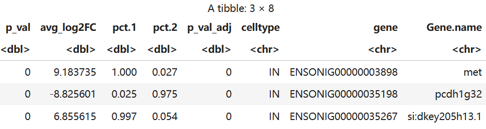
Idents(brain) <- "orig.ident"
allDEGs<-FindMarkers(
      object = brain,
      ident.1 = "TB",       # 实验组
      ident.2 = "ON",       # 对照组
      min.pct = 0.1,        # 基因在至少10%的细胞中表达
      logfc.threshold = 0.25, # 对数FC阈值
      only.pos = FALSE
    )

# 筛选显著差异基因 (按需调整阈值)
allDEGs <- allDEGs %>%
  filter(p_val_adj < 0.05 & abs(avg_log2FC) > 0.5)
找个基因查看
ON_to_TB <- read_excel("TB_TO_ON.xlsx")#TB_TO_ON.xlsx
ON.EN_to_name <- read_excel("ON.EN_to_name.xlsx")#ON.EN_to_name.xlsx
添加了一个画图功能
plot_gene_vln <- function(gene_id,
                          seurat_obj = brain,
                          tb_df = ON_to_TB,
                          on_df = ON.EN_to_name,
                          group.by = "orig.ident",
                          split.by = "CCA0.1.celltype",
                          assay = "RNA",
                          pt.size = 0.1) {
  # 提取TB名称
  tb_name <- tb_df[[2]][tb_df[[1]] == gene_id]
  if (length(tb_name) == 0) tb_name <- "Not found"
  # 提取ON名称
  on_name <- on_df[[2]][on_df[[1]] == gene_id]
  if (length(on_name) == 0) on_name <- "Not found"
  title_str <- paste0(gene_id, "  ON:", on_name, "  TB:", tb_name)
  options(repr.plot.width = 15, repr.plot.height = 5)
  # 绘制小提琴图
  p <- VlnPlot(seurat_obj,
               features = gene_id,
               group.by = group.by,
               split.by = split.by,
               assay = assay,
               pt.size = pt.size)
  # 添加标题并居中
  p + ggtitle(title_str) +
    theme(plot.title = element_text(hjust = 0.5, size = 12))
}
plot_gene_vln("ENSONIG00000012706")
Warning message:
"Groups with fewer than two datapoints have been dropped.
ℹ Set `drop = FALSE` to consider such groups for position adjustment purposes."
6.其余图片绘制
library(Seurat)
library(dplyr)
library(ggplot2)
library(tidyr)
library(patchwork)
library(Matrix)
library(harmony)
library(readxl)
library(openxlsx)
library(dplyr)

options(repr.plot.width = 6, repr.plot.height = 5)

DimPlot(brain, reduction = "umap.unintegrated", label = T, group.by =c("orig.ident"),repel = T)

DimPlot(integrated_data, reduction = "umap.unintegrated", label = T, group.by =c("CCA0.1.celltype"),repel = T)
后续分析不考虑OPCs和CPSC,因为这两类细胞类型不达标
brain <- subset(brain, subset = CCA0.1.celltype != "OPCs" & CCA0.1.celltype != "CPSC")

gene_labels <- c(
  "ENSONIG00000006551" = "etv1",
  "ENSONIG00000009548" = "grin2ca",
  "ENSONIG00000041486" = "cck",
  "ENSONIG00000018696" = "gad1b",
  "ENSONIG00000008574" = "pvalb6",
  "ENSONIG00000015427" = "lhx5",
  "ENSONIG00000010119" = "ptprc",
  "ENSONIG00000012102" = "c1ql4a",
  "ENSONIG00000013065" = "csf1ra",
  "ENSONIG00000014971" = "slc1a3a",
  "ENSONIG00000011931" = "tnc",
  "ENSONIG00000040772" = "fabp7b",
  "ENSONIG00000004332" = "plp1b",
  "ENSONIG00000014598" = "ugt8",
  "ENSONIG00000015523" = "myrf",
  "ENSONIG00000018007" = "grin2bb",
  "ENSONIG00000008933" = "tbr1b",
  "ENSONIG00000017606" = "gria1a",
  "ENSONIG00000009913" = "ptprb",
  "ENSONIG00000014676" = "slc16a1a",
  "ENSONIG00000010973" = "rgs5a",
  "ENSONIG00000035890" = "pitx2",
  "ENSONIG00000029183" = "pmch",
  "ENSONIG00000003325" = "cacna1hb",
  "ENSONIG00000001111" = "vip",
  "ENSONIG00000009878" = "sox5",
  "ENSONIG00000019914" = "mki67",
  "ENSONIG00000001324" = "cdh5",
  "ENSONIG00000020432" = "cldn5a",
  "ENSONIG00000007944" = "col1a1b",
  "ENSONIG00000016189" = "cyp4t8",
  "ENSONIG00000001051" = "tbx18",
  "ENSONIG00000003020" = "epcam",
  "ENSONIG00000003911" = "cftr",
  "ENSONIG00000015841" = "slc8a2a",
  "ENSONIG00000006405" = "foxq1b",
  "ENSONIG00000001369" = "phox2bb",
  "ENSONIG00000040944" = "trarg1"
)

p1 <- DotPlot(brain,
              features = names(gene_labels),  # 使用基因ID作为特征
              cluster.idents = TRUE,
              group.by = "CCA0.1.celltype") +
  scale_size_continuous(range = c(1, 2.5)) +
  theme(
    panel.border = element_rect(color = "black"),
    panel.spacing = unit(1, "mm"),
    strip.text = element_text(margin = margin(b = unit(3, "mm"))),
    strip.placement = "outside",
    axis.line = element_blank(),
    axis.text.x = element_text(angle = 90, vjust = 0.5, hjust = 1)  # 设置 x 轴刻度标签垂直显示
  ) +
  labs(x = "", y = "") +
  scale_color_gradientn(colours = c('
#99cfe1
','
#e6f3f8
', 'white', '
#ffbfb7
', 'red')) +
  # 设置细胞类型顺序(现在是 y 轴)
  scale_y_discrete(limits = c('EN','IN','IMM','AST','OLG','EPN','BVC','HNC','RGC','VEC', 'BBBAC', 'CPEC','CSN')) +
  # 替换基因ID为符号(现在是 x 轴)
  scale_x_discrete(labels = function(x) {
    # 使用映射向量替换标签
    ifelse(x %in% names(gene_labels), gene_labels[x], x)
  })
Scale for size is already present.
Adding another scale for size, which will replace the existing scale.
Scale for colour is already present.
Adding another scale for colour, which will replace the existing scale.
options(repr.plot.width = 12, repr.plot.height = 5)

p1

markers<-read.table("TBvsON.txt", header = TRUE)

head(markers)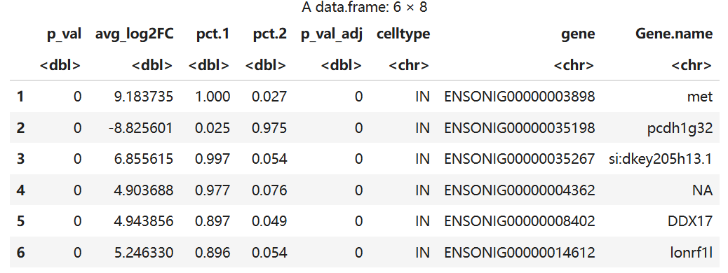
#细胞类型比例图
desired_order <- c('EN','IN','IMM','AST','OLG','EPN','BVC','HNC','RGC','VEC', 'BBBAC', 'CPEC','CSN')
brain$CCA0.1.celltype <- factor(brain$CCA0.1.celltype, levels = desired_order)
options(repr.plot.width = 7 ,repr.plot.height = 8)
colors <- c("#1fa079","#db6c18","#8a78a9","#65a51d",
            "#e6ac09","#6c6c6c", "#8cd2c6","#ffffb6","#c6c3de","#fcb5ac",
            "#8ebad7","#fdb86b","#b6de6f","#fcd2e7","#cb5768", "#6b5d99","#98757c")
ggplot(brain@meta.data,
       aes(x=orig.ident, fill=CCA0.1.celltype)) +
  geom_bar(position = "fill")+
  RotatedAxis()+theme_classic()+
  scale_fill_manual(values = colors)+
  theme(axis.text.x=element_text(angle=45,hjust = 1,vjust=1,
                                 size = 15),
        axis.text.y=element_text(size = 15),
        axis.text = element_text(color = 'black', size = 12)
  )+
  # scale_fill_gradient(low="red",high="blue")+
  labs(x=NULL,y=NULL)
查看单个基因的差异
significance_data <- subset(markers, gene == "ENSONIG00000012706")
significance_data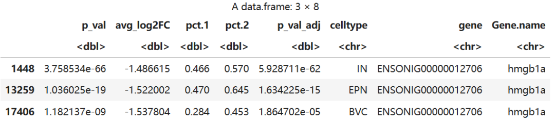
all_groups <- unique(brain@meta.data$CCA0.1.celltype)

significance_data$significance <- ifelse(significance_data$p_val_adj < 0.001, "***",
                                         ifelse(significance_data$p_val_adj < 0.01, "**",
                                                ifelse(significance_data$p_val_adj < 0.05, "*", "")))

complete_significance_data <- data.frame(
  CCA0.1.celltype = all_groups,
  significance = ifelse(all_groups %in% significance_data$celltype, significance_data$significance, "ns")
)
complete_significance_data
A data.frame: 13 × 2
CCA0.1.celltypesignificance<chr><chr>IN***ENnsRGCnsIMMnsASTnsEPN***BBBACnsBVC***HNCnsVECnsOLGnsCPECnsCSNns
VlnPlot(brain, features = c("ENSONIG00000012706"), group.by = "CCA0.1.celltype", split.by = "orig.ident", pt.size = 0.1)以此为基础可以进行后续的对于亚细胞簇的深入分析
三、参考
1.https://www.10xgenomics.com/support/software/cell-ranger/latest/tutorials/cr-tutorial-in
2.scrublet: https://github.com/AllonKleinLab/scrublet
3.https://satijalab.org/seurat/articles/integration_introduction.html
4.https://blog.csdn.net/zfyyzhys/article/details/142314175
四、资料领取
本推送的相关文件可以在以下链接中下载:

通过网盘分享的文件链接:
https://pan.baidu.com/s/1xmdzr5uJ8g_OJRKu1NY5Lg
提取码: mar6
欢迎致谢
如果以上内容对你有帮助,欢迎在文章的Acknowledgement中加上这一段,联系客服微信可以发放奖励:
Since Biomamba and his wechat public account team produce bioinformatics tutorials and share code with annotation, we thank Biomamba
for
 their guidance
in
 bioinformatics and data analysis
for
 the current study.
欢迎在发文/毕业时向我们分享你的喜悦~
已致谢文章
鼻咽癌的Bulk RNA-Seq与scRNA-Seq联合分析
13分+文章利用scRNA-Seq揭示地铁细颗粒物引起肺部炎症的分子机制
除了铁死亡,还有铜死亡?!
IF14.3| scRNA-seq+脂质组多组学分析揭示宫内生长受限导致肝损伤的性别差异银屑病和脂肪肝病中共同病理和免疫特征《Advanced Science》新型Arf1抑制剂促进癌症干细胞衰老并增强抗肿瘤免疫
scRNA-seq揭示脓毒症预后水平预测的关键靶点!
机器学习+生信多组学联合构建牙周炎"线粒体功能障碍与免疫微环境"关联网络
KIF18A在肝细胞癌转移中的双重角色
bulk+scRNA-seq挖掘BCL2-MAPK14-TXN氧化应激诊断模型,鉴定脓毒症中氧化应激关键基因
致谢文章+1,中科院1区,scRNA-seq揭示麻黄-甘草配对治疗呼吸系统症状和多(I:C)诱发肺炎模型机制
致谢文章又+1,生物信息学+机器学习鉴定驱动糖尿病肾病免疫激活和小管间隙损伤的PANoptosis枢纽基因