一、写在前面
**加权基因共表达网络分析(WGCNA)**是一类从整体层面解析转录组结构的系统生物学方法。该方法基于基因间的共表达关联构建基因网络,可将海量基因自动聚类为若干具有相似表达模式的模块,并进一步与实验分组、性状表型等变量进行关联分析,从而精准识别驱动特定生物学过程的关键模块与核心基因。
相较于传统差异表达分析仅聚焦单个基因的显著性差异,WGCNA 更注重基因间的协同表达模式,能够从网络调控视角挖掘潜在的功能单元与分子机制,在解析复杂生物性状与胁迫响应等研究中具有显著优势。
该推文主要是:对水稻在稻瘟病菌胁迫(TR)与对照(CK)的转录组数据进行整合分析,得到可靠的差异基因(Meta-DEG)与共表达模块(WGCNA),并输出可用于后续功能解释(GO/KEGG、Cytoscape网络、模块基因列表)的结果文件。总流程:CEL → RMA → PCA 质控 → probe→gene → ComBat去批次 → RankProd做Meta-DEG → 富集解释 → WGCNA 找模块 → 导出模块/网络。
二、实操流程
1 环境与路径管理
这一节只做一件事:用 here 固定项目路径,避免 RMarkdown 多个 chunk 混跑时"读不到文件/写到奇怪的地方"。
library(here)
here::i_am("rankprod_wgcna_lab_report.Rmd")
# 打印 here 认为的"项目根目录"
here::here()
1 "C:/Users/13629/Desktop/wgcna_lab_report"
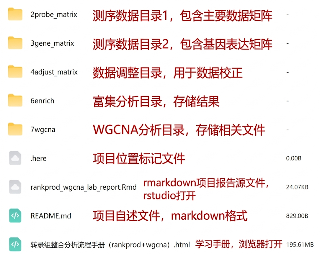
# ===== 统一目录变量 =====
DIR_RAW_GSE41798 <- here("1raw_celfile", "GSE41798_RAW")
DIR_RAW_GSE95394 <- here("1raw_celfile", "GSE95394_RAW")
DIR_PROBE_MATRIX <- here("2probe_matrix")
DIR_GENE_MATRIX  <- here("3gene_matrix")
DIR_BATCH        <- here("4adjust_matrix")   # 合并/去批次
DIR_ENRICH       <- here("6enrich")          # 富集
DIR_WGCNA        <- here("7wgcna")           # WGCNA
2 原始芯片数据标准化(RMA)与表达矩阵导出
目标:把每个 GSE 的 CEL 文件做 RMA 标准化,导出 probe-level 表达矩阵(后续再映射到基因)。
-
输入:1raw_celfile/GSE*_RAW/ 下的 CEL 文件
-
输出:2probe_matrix/GSE*_probematrix.csv
-
质控:箱线图(raw vs norm)
2.1 GSE41798:读取 CEL → RMA → 箱线图 → 导出矩阵
library(oligo)
library(affy)
# 1) 找到所有 CEL 文件
celfile <- list.celfiles(DIR_RAW_GSE41798, full.names = TRUE)
# 2) 读取 CEL
rawData <- oligo::read.celfiles(celfile)
Reading in : C:/Users/13629/Desktop/wgcna_lab_report/1raw_celfile/GSE41798_RAW/GSM1024458_Mo.CEL.gz
Reading in : C:/Users/13629/Desktop/wgcna_lab_report/1raw_celfile/GSE41798_RAW/GSM1024459_Mo.CEL.gz
Reading in : C:/Users/13629/Desktop/wgcna_lab_report/1raw_celfile/GSE41798_RAW/GSM1024460_Mo.CEL.gz
Reading in : C:/Users/13629/Desktop/wgcna_lab_report/1raw_celfile/GSE41798_RAW/GSM1024461_CK.CEL.gz
Reading in : C:/Users/13629/Desktop/wgcna_lab_report/1raw_celfile/GSE41798_RAW/GSM1024462_CK.CEL.gz
Reading in : C:/Users/13629/Desktop/wgcna_lab_report/1raw_celfile/GSE41798_RAW/GSM1024463_CK.CEL.gz
# 3) RMA 标准化(背景校正 + 分位数标准化 + summarization)
normData <- oligo::rma(rawData, background = TRUE, normalize = TRUE)
Background correcting
Normalizing
Calculating Expression
# 4) 质控:箱线图(标准化前后)
boxplot(rawData, main = "Raw intensity (GSE41798)")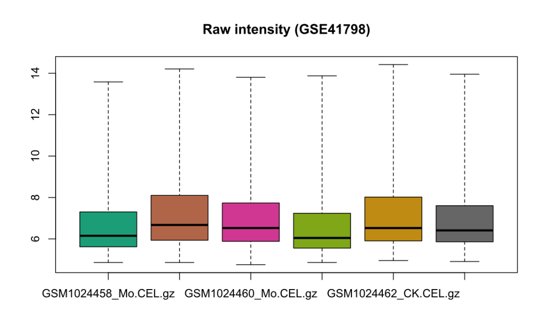
boxplot(normData, main = "RMA normalized (GSE41798)")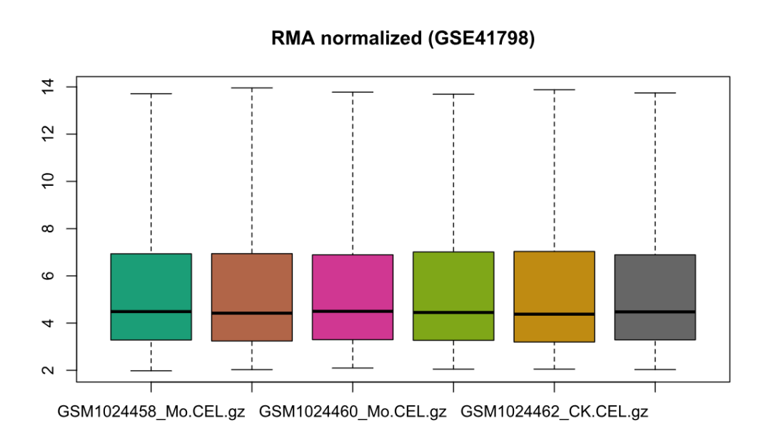
# 5) 输出 probe-level 表达矩阵到 2probe_matrix/
write.table(
  x = exprs(normData),
  file = file.path(DIR_PROBE_MATRIX, "GSE41798_probematrix.csv"),
  quote = FALSE, sep = ","
)
2.2 GSE95394:读取 CEL → RMA → 箱线图 → 导出矩阵
library(oligo)
library(affy)
celfile <- list.celfiles(DIR_RAW_GSE95394, full.names = TRUE)
rawData <- oligo::read.celfiles(celfile)
Reading in : C:/Users/13629/Desktop/wgcna_lab_report/1raw_celfile/GSE95394_RAW/GSM2509722_Mo.CEL.gz
Reading in : C:/Users/13629/Desktop/wgcna_lab_report/1raw_celfile/GSE95394_RAW/GSM2509723_Mo.CEL.gz
Reading in : C:/Users/13629/Desktop/wgcna_lab_report/1raw_celfile/GSE95394_RAW/GSM2509724_Mo.CEL.gz
Reading in : C:/Users/13629/Desktop/wgcna_lab_report/1raw_celfile/GSE95394_RAW/GSM2509725_CK.CEL.gz
Reading in : C:/Users/13629/Desktop/wgcna_lab_report/1raw_celfile/GSE95394_RAW/GSM2509726_CK.CEL.gz
Reading in : C:/Users/13629/Desktop/wgcna_lab_report/1raw_celfile/GSE95394_RAW/GSM2509727_CK.CEL.gz
normData <- oligo::rma(rawData, background = TRUE, normalize = TRUE)Background correcting
Normalizing
Calculating Expression
boxplot(rawData, main = "Raw intensity (GSE95394)")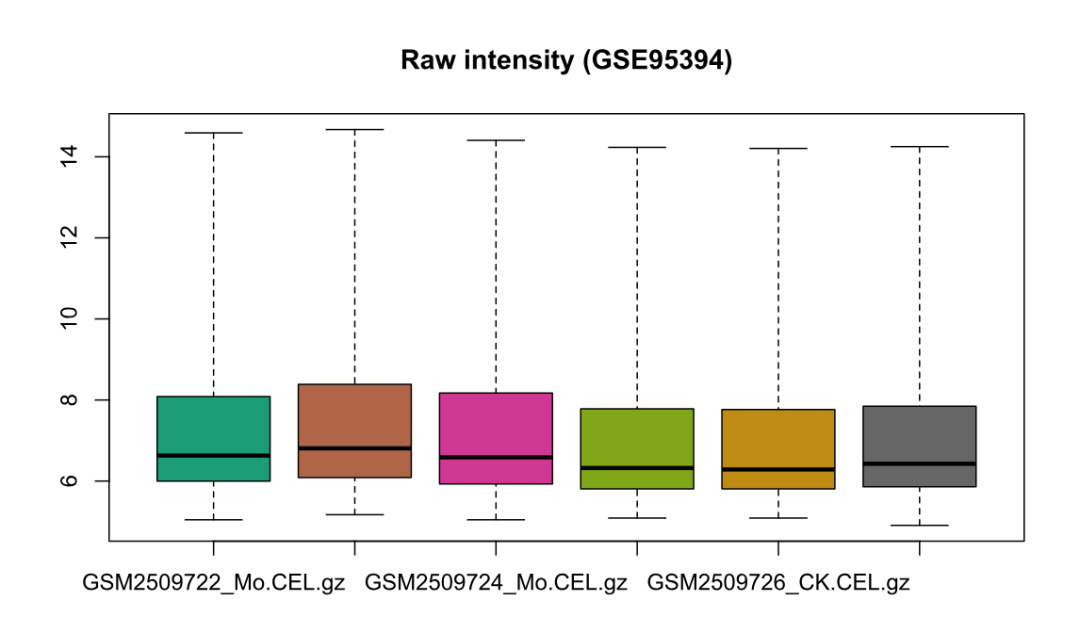
boxplot(normData, main = "RMA normalized (GSE95394)")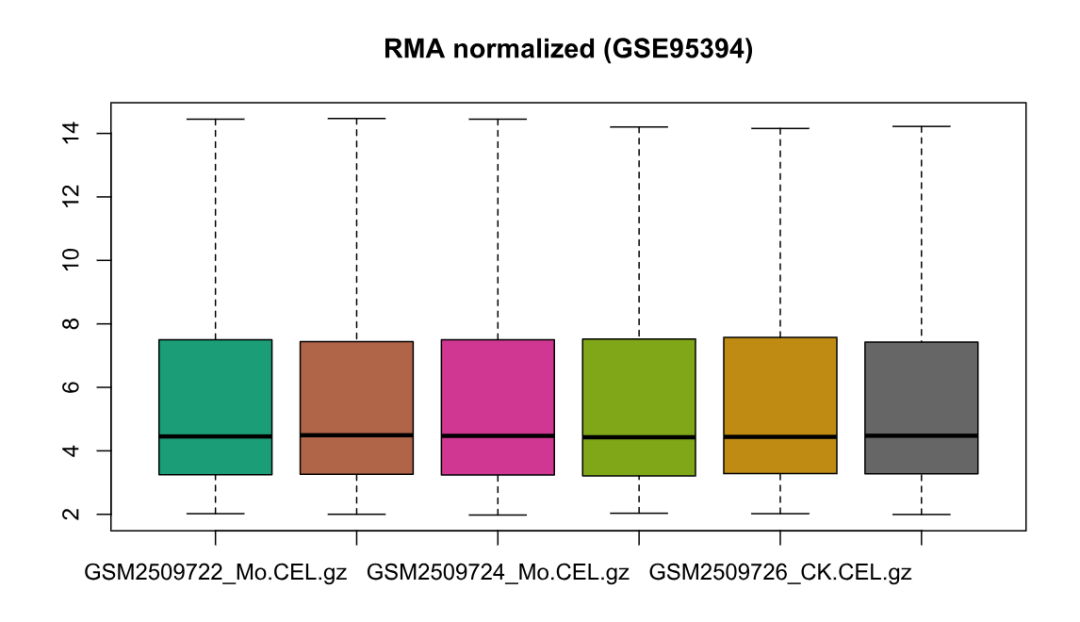
write.table(
  x = exprs(normData),
  file = file.path(DIR_PROBE_MATRIX, "GSE95394_probematrix.csv"),
  quote = FALSE, sep = ","
)
3 PCA:检查分组与批次效应是否存在
目标:用 PCA 快速判断
1)分组文件长度是否和表达矩阵样本数一致
2)样本是否离群
3)后续合并时批次效应是否明显
如何读图:点之间越近→表达谱越相似;越远→差异越大。
如果按 Group(CK/TR)上色后分开明显→胁迫信号强;如果按 Batch 分团明显→批次效应强,需要 ComBat。
3.1 GSE41798 PCA(检查 Group 与样本列名是否对齐)
library(ggord)
exprs <- read.table(file.path(DIR_PROBE_MATRIX, "GSE41798_probematrix.csv"),
                    row.names = 1, header = TRUE, sep = ",", check.names = FALSE)
group <- read.table(file.path(DIR_PROBE_MATRIX, "GSE41798_group.txt"),
                    header = TRUE, sep = "\t")
# 0) 基础一致性检查:列数=分组长度
cat("expr samples:", ncol(exprs), "\n")
expr samples: 6
cat("group length :", nrow(group), "\n")group length : 6
# 1) 去除全 0 行(极少数数据会出现)
exprs2 <- exprs[rowSums(exprs) > 0, , drop = FALSE]
# 2) PCA:样本在行、特征在列,因此要转置
pca_data <- t(as.matrix(exprs2))
pca1 <- prcomp(pca_data, center = TRUE, scale. = TRUE)
# 3) 画图:按 Group 上色
pca_group <- factor(group$Group)
ggord(pca1, grp_in = pca_group, txt = NULL, vec_ext = 0, arrow = 0,
      hull = FALSE, ellipse = TRUE, obslab = FALSE, size = 2)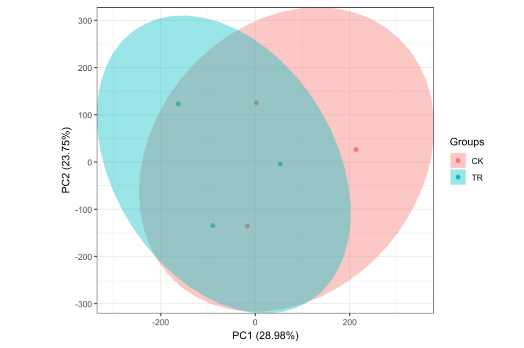
3.2 GSE95394 PCA
library(ggord)
exprs <- read.table(file.path(DIR_PROBE_MATRIX, "GSE95394_probematrix.csv"),
                    row.names = 1, header = TRUE, sep = ",", check.names = FALSE)
group <- read.table(file.path(DIR_PROBE_MATRIX, "GSE95394_group.txt"),
                    header = TRUE, sep = "\t")
cat("expr samples:", ncol(exprs), "\n")
expr samples: 6
cat("group length :", nrow(group), "\n")group length : 6
exprs2 <- exprs[rowSums(exprs) > 0, , drop = FALSE]
pca_data <- t(as.matrix(exprs2))
pca1 <- prcomp(pca_data, center = TRUE, scale. = TRUE)
pca_group <- factor(group$Group)
ggord(pca1, grp_in = pca_group, txt = NULL, vec_ext = 0, arrow = 0,
      hull = FALSE, ellipse = TRUE, obslab = FALSE, size = 2)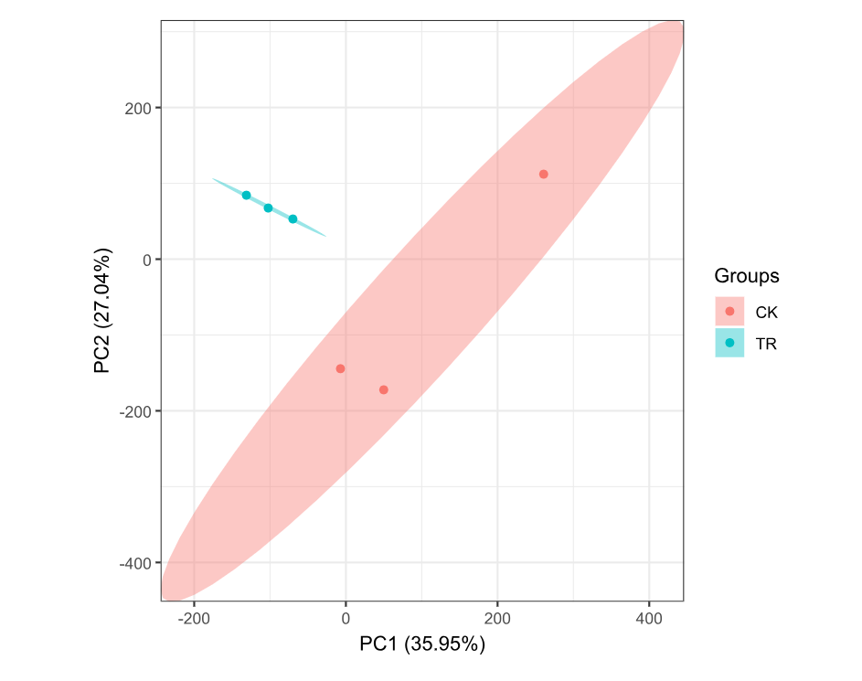
4 探针(probe)映射到基因(gene)并合并重复探针
芯片数据通常是 probe-level,后续做整合分析更推荐 gene-level。
本节做两件事:
1)用 probe2geneid.csv 把 probe 映射到 gene
2)同一 gene 多个 probe 时用平均值合并(mean)
输出:
-
4adjust_matrix/GSE41798_genematrix.csv
-
4adjust_matrix/GSE95394_genematrix.csv
library(dplyr)
1) 读取探针-基因映射表
idmap <- read.csv(file.path(DIR_GENE_MATRIX, "probe2geneid.csv"), header = TRUE)
2) 读取 probe-level 表达矩阵(注意:来自 2probe_matrix)
matrix <- read.csv(file.path(DIR_PROBE_MATRIX, "GSE41798_probematrix.csv"), check.names = FALSE)
把行名(探针ID)变成一列 Probe_ID,才能 merge
matrix <- cbind(Probe_ID = rownames(matrix), matrix)
rownames(matrix) <- NULL3) 合并:把 Gene_ID 加到表达矩阵里
exprSet <- merge(idmap, matrix, by = "Probe_ID")
exprSet <- exprSet %>% arrange(Gene_ID)4) 对同一 Gene 的多 probe 做均值汇总
exprSet_mergeID <- aggregate(
x = exprSet[, 3:ncol(exprSet)],
by = list(exprSet$Gene_ID),
FUN = mean
)5) 输出到 4adjust_matrix/
out_file <- file.path(DIR_BATCH, "GSE41798_genematrix.csv")
write.table(exprSet_mergeID, file = out_file, sep = ",",
row.names = FALSE, quote = FALSE)library(dplyr)
idmap <- read.csv(file.path(DIR_GENE_MATRIX, "probe2geneid.csv"), header = TRUE)
matrix <- read.csv(file.path(DIR_PROBE_MATRIX, "GSE95394_probematrix.csv"), check.names = FALSE)
matrix <- cbind(Probe_ID = rownames(matrix), matrix)
rownames(matrix) <- NULL
exprSet <- merge(idmap, matrix, by = "Probe_ID")
exprSet <- exprSet %>% arrange(Gene_ID)
exprSet_mergeID <- aggregate(
x = exprSet[, 3:ncol(exprSet)],
by = list(exprSet$Gene_ID),
FUN = mean
)
out_file <- file.path(DIR_BATCH, "GSE95394_genematrix.csv")
write.table(exprSet_mergeID, file = out_file, sep = ",",
row.names = FALSE, quote = FALSE)
5 合并两组数据并用 ComBat 去除批次效应
目标:
1)合并两组 gene-level 矩阵
2)PCA 检测批次效应
3)ComBat 去批次后再 PCA 验证
输出:
-
combine_matrix.csv
-
adjusted_matrix.csv
library(ggord)
library(ggplot2)
library(sva)
# 1) 读取两组 gene-level 矩阵
a <- read.csv(file.path(DIR_BATCH, "GSE41798_genematrix.csv"), header = TRUE)
b <- read.csv(file.path(DIR_BATCH, "GSE95394_genematrix.csv"), header = TRUE)
# 2) 合并:按 Gene_ID(这里在你的数据里列名叫 Group.1)
combine_ab <- merge(a, b, by = "Group.1")
write.csv(combine_ab, file = file.path(DIR_BATCH, "combine_matrix.csv"),
row.names = FALSE, quote = FALSE)
# 3) PCA:去批次前
exprs <- read.csv(file.path(DIR_BATCH, "combine_matrix.csv"),
header = TRUE, row.names = 1, sep = ",")
group <- read.table(file.path(DIR_BATCH, "combine_group.txt"),
header = TRUE, sep = "\t")
# 关键:按样本名把 group 对齐到表达矩阵列顺序(避免错位导致"假批次/假生物差异")
group <- group[match(colnames(exprs), group$Sample), ]
stopifnot(ncol(exprs) == nrow(group))
pca_group <- factor(group$Batch)   # 批次信息
pca_data <- t(as.matrix(exprs))
pca1 <- prcomp(pca_data, center = TRUE, retx = TRUE, scale. = TRUE)
p1 <- ggord(pca1, grp_in = pca_group, txt = NULL, vec_ext = 0, arrow = 0,
            hull = FALSE, ellipse = FALSE, obslab = FALSE,
            size = 3, xlims = c(-300, 300), ylims = c(-200, 200))
print(p1)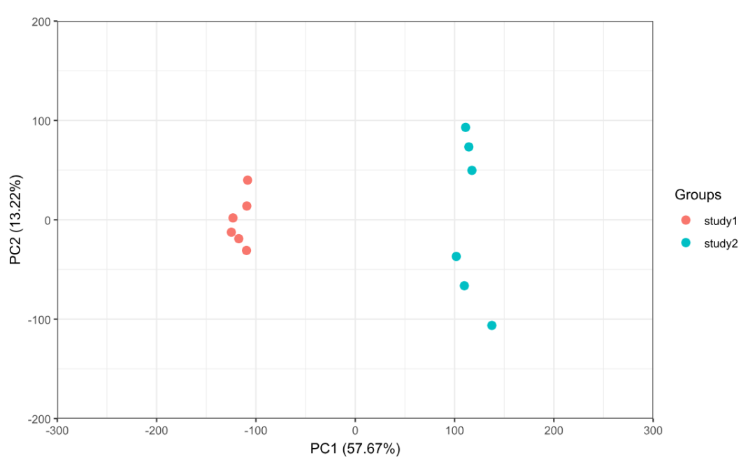
# 4) ComBat 去批次
adjusted <- ComBat(dat = exprs, batch = group$Batch, mod = NULL)
# 输出到 4adjust_matrix/
write.csv(adjusted, file = file.path(DIR_BATCH, "adjusted_matrix.csv"), quote = FALSE)
# 同时复制一份到 7wgcna/,方便后面直接用
write.csv(adjusted, file = file.path(DIR_WGCNA, "adjusted_matrix.csv"), quote = FALSE)
# 5) 去批次后 PCA(理想情况:不同 batch 更混合)
pca_data1 <- t(as.matrix(adjusted))
pca_after <- prcomp(pca_data1, center = TRUE, retx = TRUE, scale. = TRUE)
p2 <- ggord(pca_after, grp_in = pca_group, txt = NULL, vec_ext = 0, arrow = 0,
            hull = FALSE, ellipse = FALSE, obslab = FALSE,
            size = 3, xlims = c(-300, 300), ylims = c(-200, 200))
print(p2)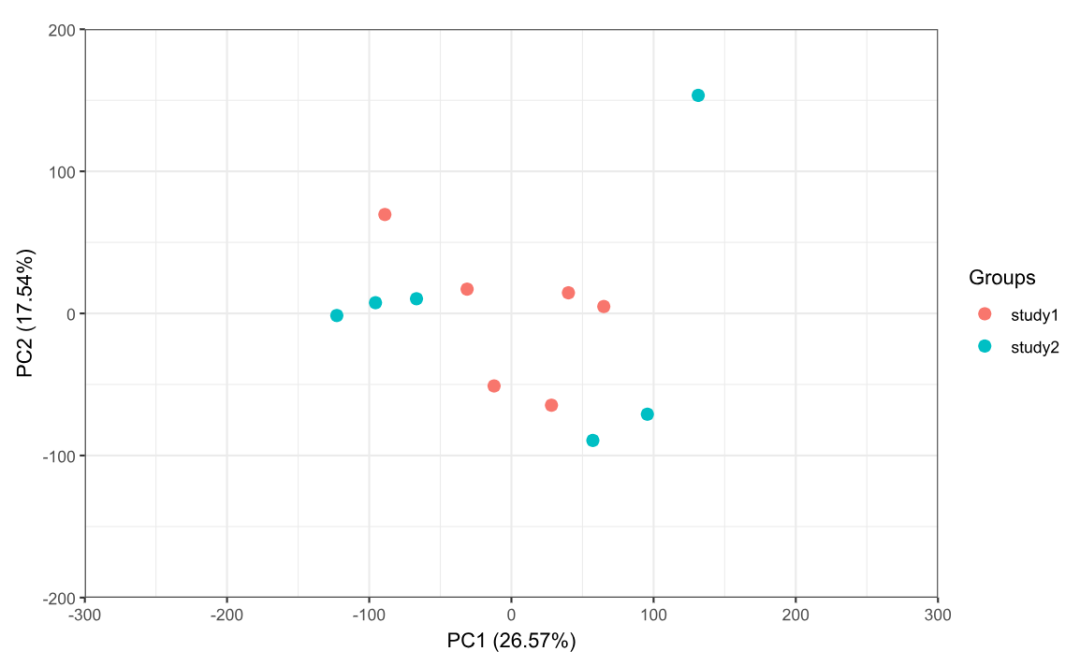
6 RankProd:单研究 DEG + Meta-DEG
目标:在多研究/多批次背景下做稳健差异基因(Meta-DEG)
输出:
-
study1-upresult.csv / study1-downresult.csv
-
study2-upresult.csv / study2-downresult.csv
-
meta-upresult.csv / meta-downresult.csv
关键输入(必须与表达矩阵列顺序一一对应):
-
class:每个样本的条件标签(TR=1,CK=0)
-
origin:每个样本属于哪个 study(study1=1,study2=2)
library(Rmpfr)
library(RankProd)
data <- read.csv(file.path(DIR_BATCH, "adjusted_matrix.csv"),
header = TRUE, row.names = 1, check.names = FALSE)=========================================================
重要:下面是"示例写法"
你只需要保证:length(class) == length(origin) == ncol(data)
且它们的顺序与 colnames(data) 完全一致
=========================================================
class <- c(rep(1,3), rep(0,3), rep(1,3), rep(0,3)) # TR=1, CK=0
origin <- c(rep(1,6), rep(2,6)) # study1=1, study2=2
geneid <- rownames(data)
stopifnot(length(class) == ncol(data))
stopifnot(length(origin) == ncol(data))单研究 DEG
for (k in1:2) {
data.sub <- data[, which(origin == k)]
class.sub <- class[which(origin == k)]
RP.out <- RankProducts(data.sub, class.sub,
logged = TRUE,
na.rm = FALSE,
plot = FALSE,
rand = 123)可视化:PFP cutoff 0.05
plotRP(RP.out, cutoff = 0.05)
ind_result <- topGene(RP.out, cutoff = 0.05, method = "pfp",
                      logged = TRUE, logbase = 2, gene.names = geneid)
write.csv(ind_result$Table1, file = paste0("study", k, "-upresult.csv"))
write.csv(ind_result$Table2, file = paste0("study", k, "-downresult.csv"))
}
Rank Product analysis for unpaired case
done
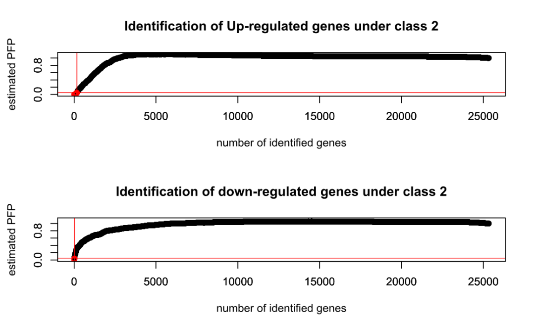
Table1: Genes called significant under class1 < class2
Table2: Genes called significant under class1 > class2
Rank Product analysis for unpaired case
done
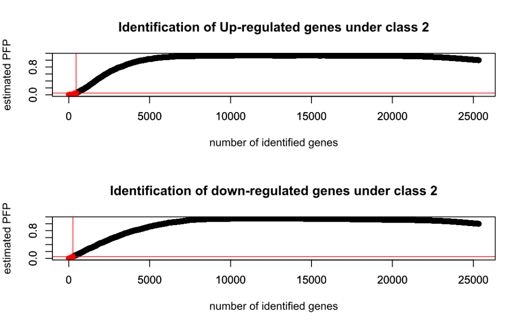
Table1: Genes called significant under class1 < class2
Table2: Genes called significant under class1 > class2
# Meta-DEG(跨研究)
RP.adv.out <- RP.advance(data, class, origin, logged = TRUE,
                         gene.names = geneid, rand = 123)
The data is from 2 different origins
Rank Product analysis for two-class case
Rank Product analysis for unpaired case
Rank Product analysis for unpaired case
done
plotRP(RP.adv.out, cutoff = 0.05)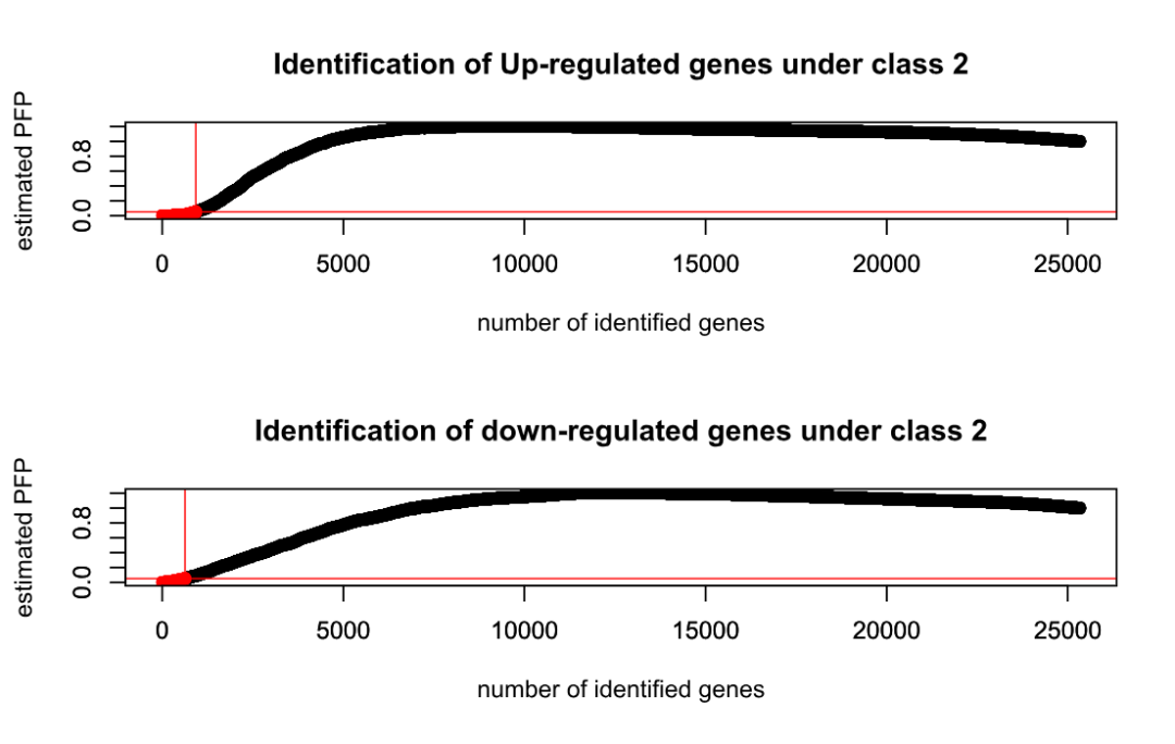
meta_DEG <- topGene(RP.adv.out, cutoff = 0.05, method = "pfp",
logged = TRUE, logbase = 2, gene.names = geneid)
Table1: Genes called significant under class1 < class2
Table2: Genes called significant under class1 > class2
write.csv(meta_DEG$Table1, file = "meta-upresult.csv")
write.csv(meta_DEG$Table2, file = "meta-downresult.csv")
7 富集分析:把 DEG "翻译成生物学含义"
输入:meta-downid.txt(一列基因 ID,无表头)
输出:
downmeta_bpresult.csv/downmeta_mfresult.csv/ downmeta_ccresult.csv
downmeta_koresult.csv
富集依赖注释文件(你已经准备了),但不同版本注释字段可能不一致。
因此这部分我加了"小检查函数",如果 level 字段不是 BP/MF/CC,会提示你实际是什么。
library(clusterProfiler)
KOannotation <- read.delim(file.path(DIR_ENRICH, "OsKOannotation08.tsv"), stringsAsFactors = FALSE)
GOannotation <- read.delim(file.path(DIR_ENRICH, "OsGOannotation08.tsv"), stringsAsFactors = FALSE)
GOinfo       <- read.delim(file.path(DIR_ENRICH, "go.tb"), stringsAsFactors = FALSE)
GOannotation1 <- split(GOannotation, with(GOannotation, level))
gene_list <- read.table(file.path(DIR_ENRICH, "meta-downid.txt"),
                        header = FALSE, check.names = FALSE)
gene <- as.character(gene_list[, 1])
# 小工具:兼容 level 可能是 "MF" 或 "molecular_function" 等写法
get_level_df <- function(go_list, key_short, key_long) {
if (!is.null(go_list[[key_short]])) return(go_list[[key_short]])
if (!is.null(go_list[[key_long]]))  return(go_list[[key_long]])
  stop(paste0("在 GOannotation 的 level 里找不到:", key_short, " 或 ", key_long,
"。请先 table(GOannotation$level) 看看实际叫什么。"))
}
MF_df <- get_level_df(GOannotation1, "MF", "molecular_function")
CC_df <- get_level_df(GOannotation1, "CC", "cellular_component")
BP_df <- get_level_df(GOannotation1, "BP", "biological_process")
MF_result <- enricher(gene, TERM2GENE = MF_df[c(2, 1)], TERM2NAME = GOinfo[1:2])
CC_result <- enricher(gene, TERM2GENE = CC_df[c(2, 1)], TERM2NAME = GOinfo[1:2])
BP_result <- enricher(gene, TERM2GENE = BP_df[c(2, 1)], TERM2NAME = GOinfo[1:2])
dotplot(BP_result, showCategory = 20)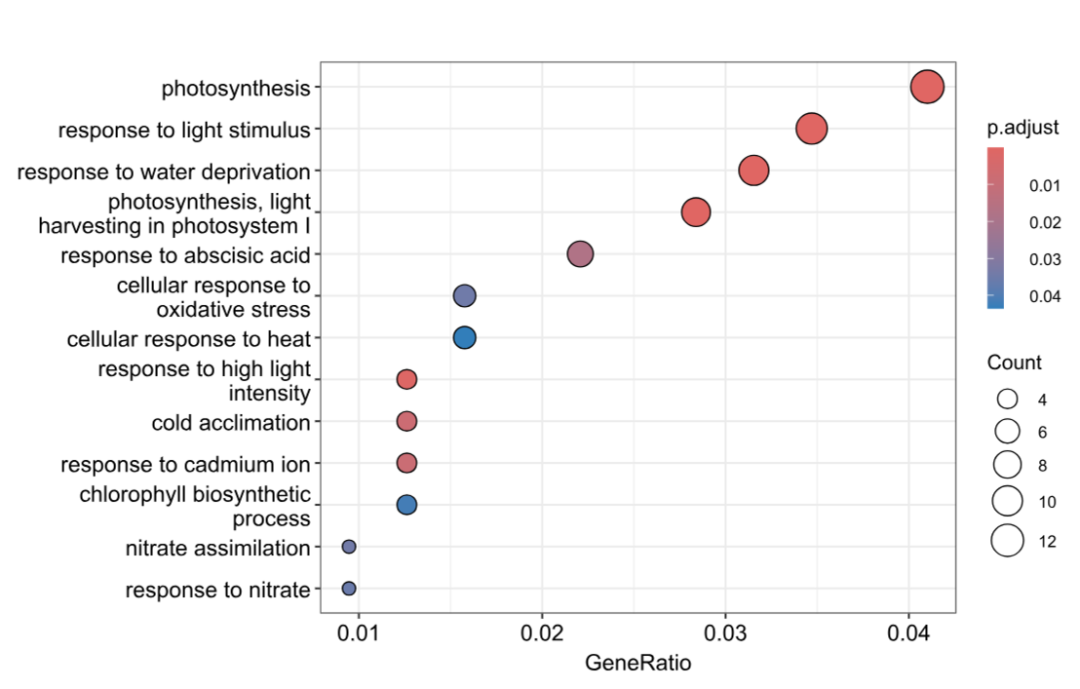
dotplot(MF_result, showCategory = 10)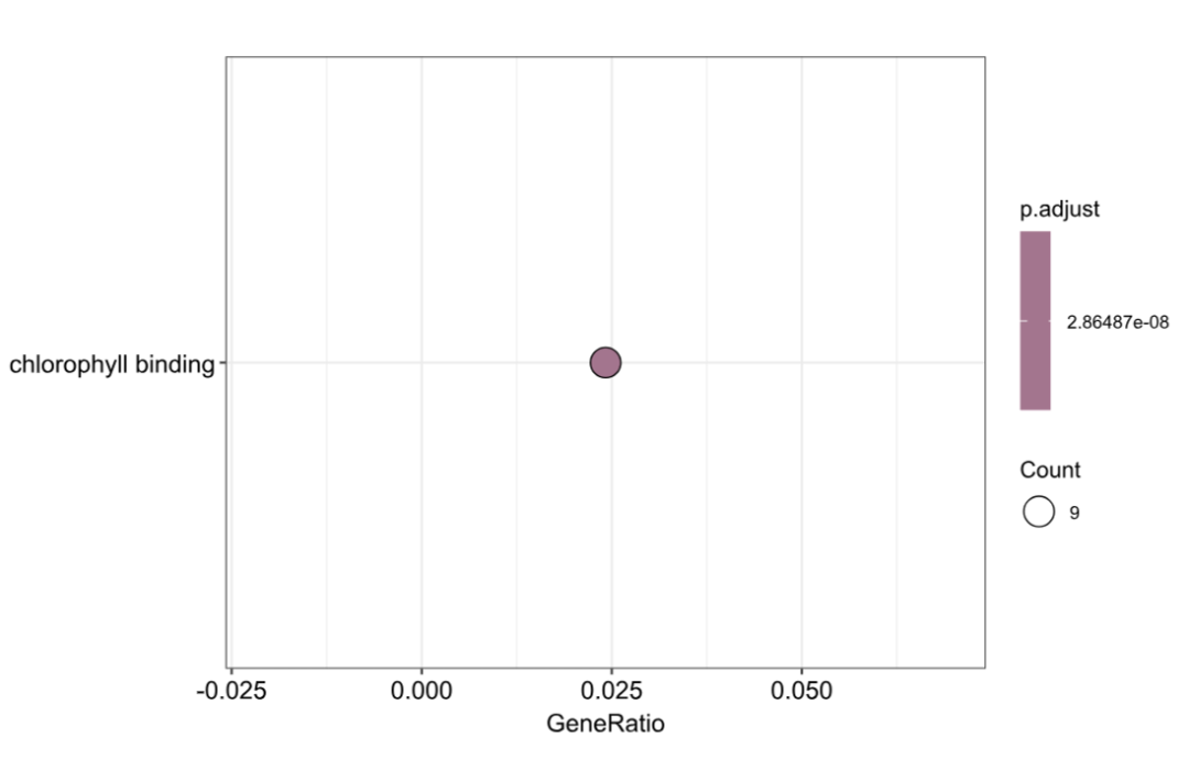
dotplot(CC_result, showCategory = 10)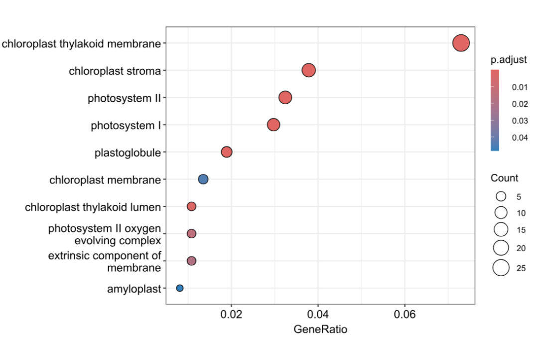
write.csv(as.data.frame(BP_result), file = "downmeta_bpresult.csv", row.names = FALSE)
write.csv(as.data.frame(MF_result), file = "downmeta_mfresult.csv", row.names = FALSE)
write.csv(as.data.frame(CC_result), file = "downmeta_ccresult.csv", row.names = FALSE)
KO_result <- enricher(gene, TERM2GENE = KOannotation[c(3, 1)], TERM2NAME = KOannotation[c(3, 4)])
dotplot(KO_result, showCategory = 10)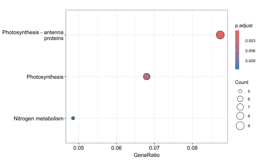
write.csv(as.data.frame(KO_result), file = "downmeta_koresult.csv", row.names = FALSE)8 WGCNA:构建共表达网络并识别模块
这一节完成:
-
数据前处理(MAD 过滤、剔除坏样本/坏基因)
-
选择 soft-threshold power
-
构网 → 切模块 → 合并模块
-
模块-性状相关热图
-
导出模块基因列表与 Cytoscape 网络文件
8.1 数据前处理 + trait 对齐
library(WGCNA)
# 多线程(不同版本函数名可能不同;allowWGCNAThreads 兼容性相对好)
allowWGCNAThreads(nThreads = parallel::detectCores())
Allowing multi-threading with up to 16 threads.
# 读取去批次后的表达矩阵(基因 × 样本)
datExpr <- read.csv(file.path(DIR_WGCNA, "adjusted_matrix.csv"), check.names = FALSE)
# 常见情况:第一列被读成 "X"(基因 ID)
rownames(datExpr) <- datExpr$X
datExpr$X <- NULL
# 强制转数值型(WGCNA 对字符/因子非常敏感)
datExpr[] <- lapply(datExpr, function(x) as.numeric(as.character(x)))
datExpr <- as.data.frame(datExpr)
# MAD 过滤:保留变化大的基因(降低噪声与计算量)
m.mad   <- apply(datExpr, 1, mad, na.rm = TRUE)
mad_cut <- max(quantile(m.mad, probs = 0.5, na.rm = TRUE), 0.01)
ExprVar <- datExpr[m.mad > mad_cut, ]
cat("genes after MAD filter:", nrow(ExprVar), "\n")
genes after MAD filter: 12666
# WGCNA 要求:样本在行、基因在列
ExprVar <- as.data.frame(t(ExprVar))
# 质量控制:剔除坏样本/坏基因
gsg <- goodSamplesGenes(ExprVar, verbose = 3)
Flagging genes and samples with too many missing values...
..step 1
..Excluding 1 samples from the calculation due to too many missing genes.
..step 2
if (!gsg$allOK) {
  ExprVar <- ExprVar[gsg$goodSamples, gsg$goodGenes]
}
# 读取性状表(行=样本)
datTraits <- read.csv(file.path(DIR_WGCNA, "trait.csv"), check.names = FALSE)
rownames(datTraits) <- datTraits$sample.ID
datTraits$sample.ID <- NULL
# 对齐样本顺序(避免 "模块-性状相关" 被错位污染)
commonSamples <- intersect(rownames(ExprVar), rownames(datTraits))
ExprVar    <- ExprVar[commonSamples, , drop = FALSE]
datTraits  <- datTraits[commonSamples, , drop = FALSE]
stopifnot(all(rownames(datTraits) == rownames(ExprVar)))
save(ExprVar, datTraits, file = file.path(DIR_WGCNA, "expr+trait.RData"))
8.2 选择 soft-threshold power
library(WGCNA)
load(file.path(DIR_WGCNA, "expr+trait.RData"))
allowWGCNAThreads(nThreads = parallel::detectCores())
Allowing multi-threading with up to 16 threads.
powers <- 1:20
sft <- pickSoftThreshold(ExprVar, powerVector = powers, verbose = 5)
pickSoftThreshold: will use block size 3532.
pickSoftThreshold: calculating connectivity for given powers...
..working on genes 1 through 3532 of 12666
..working on genes 3533 through 7064 of 12666
..working on genes 7065 through 10596 of 12666
..working on genes 10597 through 12666 of 12666
Power SFT.R.sq slope truncated.R.sq mean.k. median.k. max.k.
1 1 0.5530 2.790 0.923 4740.0 4800.0 6730
2 2 0.1360 0.538 0.823 2480.0 2430.0 4520
3 3 0.0787 -0.290 0.788 1510.0 1400.0 3330
4 4 0.3890 -0.690 0.840 1000.0 879.0 2590
5 5 0.5650 -0.938 0.879 703.0 583.0 2080
6 6 0.6540 -1.120 0.892 515.0 405.0 1710
7 7 0.7070 -1.230 0.913 389.0 290.0 1440
8 8 0.7240 -1.340 0.913 302.0 214.0 1220
9 9 0.7470 -1.410 0.921 239.0 162.0 1060
10 10 0.7530 -1.480 0.920 193.0 125.0 919
11 11 0.7750 -1.520 0.934 158.0 97.8 808
12 12 0.7930 -1.560 0.944 131.0 77.7 715
13 13 0.8080 -1.590 0.952 109.0 62.7 638
14 14 0.8160 -1.610 0.956 92.4 51.2 572
15 15 0.8170 -1.650 0.956 78.7 42.1 516
16 16 0.8210 -1.670 0.956 67.6 35.0 467
17 17 0.8310 -1.680 0.963 58.5 29.4 425
18 18 0.8400 -1.690 0.968 51.0 24.8 389
19 19 0.8490 -1.700 0.971 44.6 21.2 356
20 20 0.8590 -1.710 0.976 39.3 18.1 328
par(mfrow = c(1,2), mar = c(5.5,4.1,4.1,2.1))
cex1 <- 0.6
# (1) Scale-free 拟合度(signed R^2)
plot(sft$fitIndices[,1], -sign(sft$fitIndices[,3])*sft$fitIndices[,2],
xlab="Soft Threshold (power)",
ylab="Scale Free Topology Model Fit,signed R^2",
type="n",
main = "Scale independence")
text(sft$fitIndices[,1], -sign(sft$fitIndices[,3])*sft$fitIndices[,2],
labels=powers, cex=cex1, col="red")
abline(h=0.85, col="red")  # 常用参考阈值,可自调
# (2) 平均连接度
plot(sft$fitIndices[,1], sft$fitIndices[,5],
xlab="Soft Threshold (power)",
ylab="Mean Connectivity",
type="n",
main="Mean connectivity")
text(sft$fitIndices[,1], sft$fitIndices[,5],
labels=powers, cex=cex1, col="red")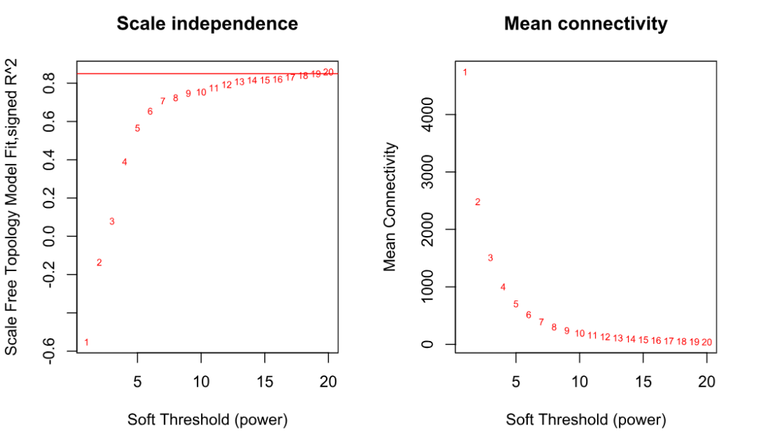
经验规则:选一个让 R^2 接近/超过 0.85,同时 mean connectivity 不至于太低的 power
8.3 构网、切模块、合并模块(并把关键对象保存下来)
library(WGCNA)
load(file.path(DIR_WGCNA, "expr+trait.RData"))
# 你可以把这里替换成你自己从上一步图里选的 power
softPower <- 11
# 1) 邻接矩阵(基因-基因相似)
adjacency <- adjacency(ExprVar, power = softPower)
# 2) TOM 相似度(更稳健的"网络相似度")
tom_sim <- TOMsimilarity(adjacency)
..connectivity..
..matrix multiplication (system BLAS)..
..normalization..
..done.
dimnames(tom_sim) <- dimnames(adjacency)
tom_dis <- 1 - tom_sim
# 3) 基因聚类树
geneTree <- hclust(as.dist(tom_dis), method = "average")
plot(geneTree, xlab = "", sub = "", main = "Gene clustering (TOM dissimilarity)",
labels = FALSE, hang = 0.04)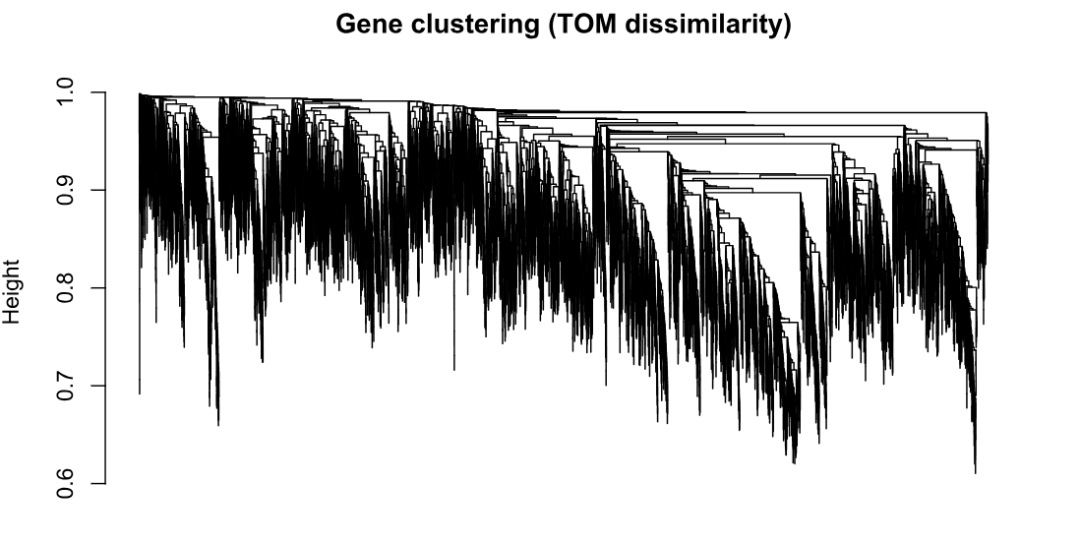
# 4) 动态剪切得到初始模块
minModuleSize <- 150
dynamicMods <- cutreeDynamic(dendro = geneTree, distM = tom_dis,
deepSplit = 2, pamRespectsDendro = FALSE,
minClusterSize = minModuleSize)
..cutHeight not given, setting it to 0.996 ===> 99% of the (truncated) height range in dendro.
..done.
dynamicColors <- labels2colors(dynamicMods)
plotDendroAndColors(geneTree, dynamicColors, "Dynamic Tree Cut",
dendroLabels = FALSE, addGuide = TRUE,
hang = 0.03, guideHang = 0.05)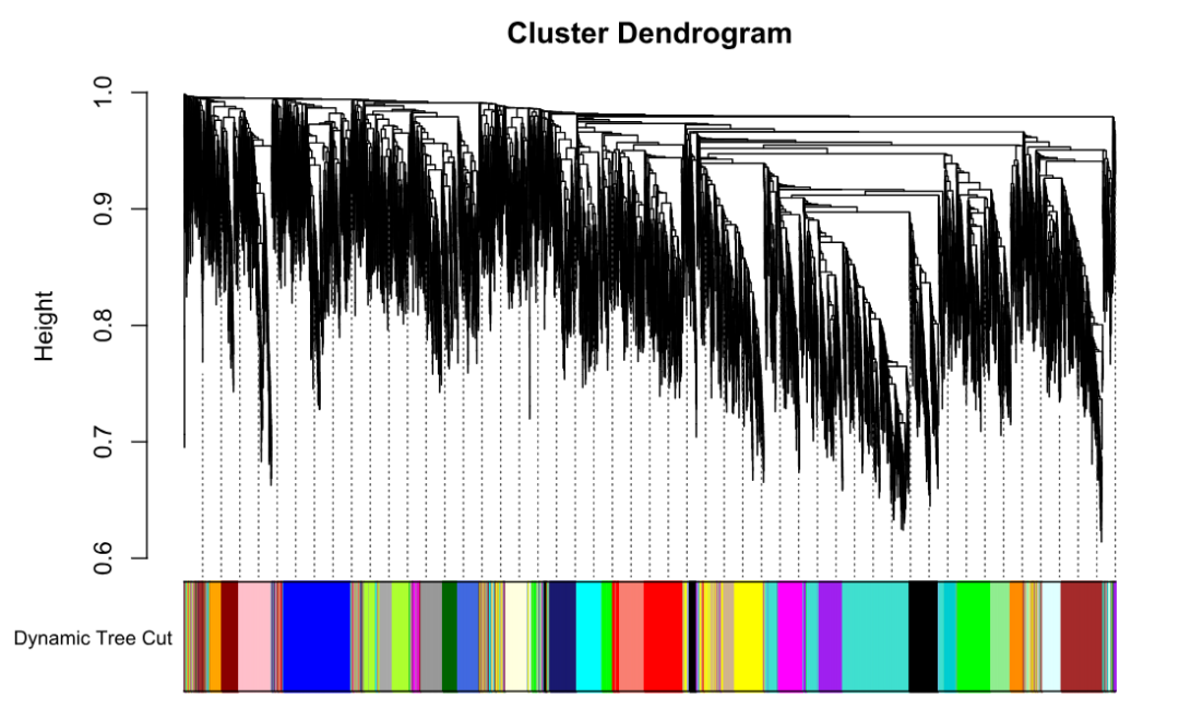
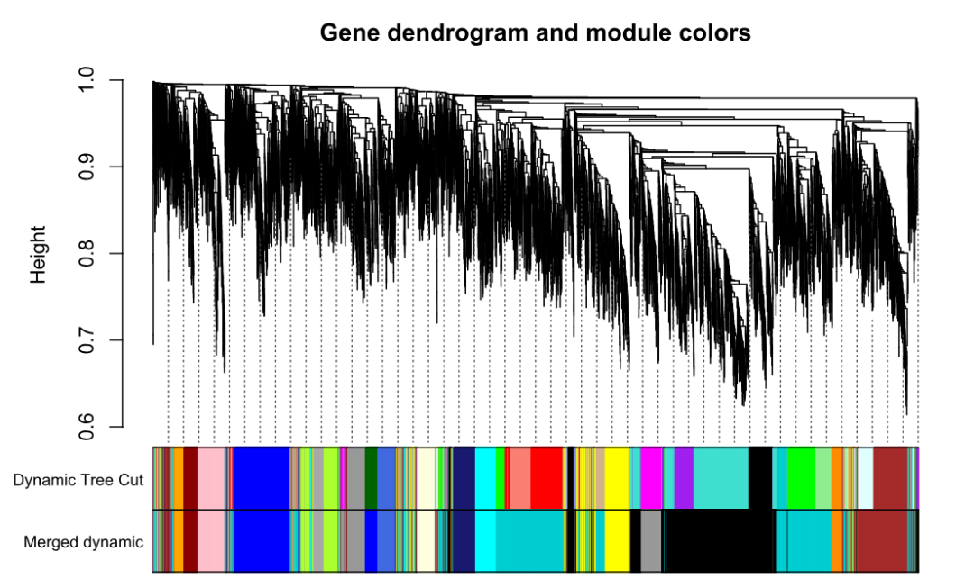
# 5) 合并相似模块(cutHeight 越小合并越少)
merge_module <- mergeCloseModules(ExprVar, dynamicColors,
cutHeight = 0.2, verbose = 3)
mergeCloseModules: Merging modules whose distance is less than 0.2
multiSetMEs: Calculating module MEs.
Working on set 1 ...
moduleEigengenes: Calculating 27 module eigengenes in given set.
multiSetMEs: Calculating module MEs.
Working on set 1 ...
moduleEigengenes: Calculating 19 module eigengenes in given set.
multiSetMEs: Calculating module MEs.
Working on set 1 ...
moduleEigengenes: Calculating 18 module eigengenes in given set.
multiSetMEs: Calculating module MEs.
Working on set 1 ...
moduleEigengenes: Calculating 17 module eigengenes in given set.
Calculating new MEs...
multiSetMEs: Calculating module MEs.
Working on set 1 ...
moduleEigengenes: Calculating 17 module eigengenes in given set.
mergedColors <- merge_module$colors
mergedMEs    <- merge_module$newMEs
plotDendroAndColors(
  geneTree,
cbind(dynamicColors, mergedColors),
c("Dynamic Tree Cut", "Merged dynamic"),
  dendroLabels = FALSE, addGuide = TRUE,
  hang = 0.03, guideHang = 0.05,
  main = "Gene dendrogram and module colors"
)
# 保存:后面导热图/导出 Cytoscape 都要用到
save(geneTree, tom_sim, mergedColors, mergedMEs, merge_module,
file = file.path(DIR_WGCNA, "wgcna_network.RData"))
8.4 模块与性状相关热图
library(WGCNA)
load(file.path(DIR_WGCNA, "expr+trait.RData"))
load(file.path(DIR_WGCNA, "wgcna_network.RData"))
moduleTraitCor <- cor(mergedMEs, datTraits, use = "p")
moduleTraitPvalue <- corPvalueStudent(moduleTraitCor, nSamples = nrow(ExprVar))
textMatrix <- paste(signif(moduleTraitCor, 2), "\n(",
signif(moduleTraitPvalue, 1), ")", sep = "")
dim(textMatrix) <- dim(moduleTraitCor)
par(mar = c(3, 10, 2, 2))
labeledHeatmap(Matrix = moduleTraitCor,
main = "Module-trait relationships",
xLabels = names(datTraits),
yLabels = names(mergedMEs),
ySymbols = names(mergedMEs),
colorLabels = FALSE,
colors = blueWhiteRed(50),
cex.text = 0.6,
cex.axis = 0.6,
zlim = c(-1, 1),
xLabelsAngle = 45,
textMatrix = textMatrix,
setStdMargins = FALSE)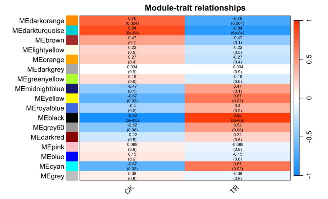
8.5 导出模块基因列表与 Cytoscape 网络
8.5.1 输出每个模块的基因(grey 通常为未分配模块)
load(file.path(DIR_WGCNA, "expr+trait.RData"))
load(file.path(DIR_WGCNA, "wgcna_network.RData"))
probes <- colnames(ExprVar)
mods <- names(table(mergedColors))
for (modules in mods) {
  inModule <- (mergedColors == modules)
  modGenes <- probes[inModule]
  write.table(modGenes,
file = paste0(modules, ".txt"),
              sep = "\t",
              row.names = FALSE, col.names = FALSE, quote = FALSE)
}
8.5.2 导出 Cytoscape 网络文件(按模块)
load(file.path(DIR_WGCNA, "expr+trait.RData"))
load(file.path(DIR_WGCNA, "wgcna_network.RData"))
probes <- colnames(ExprVar)
mods2 <- unique(mergedColors)
mods2 <- mods2[mods2 != "grey"]
mods2 <- mods2[!is.na(mods2)]
n <- length(mods2)
pb <- txtProgressBar(min = 0, max = n, style = 3)
| | | 0%
for (p in seq_len(n)) {
modules <- mods2[p]
  inModule <- (mergedColors == modules)
  modProbes <- probes[inModule]
  modTOM <- tom_sim[inModule, inModule]
  dimnames(modTOM) <- list(modProbes, modProbes)
# 阈值:取 TOM 的 0.8 分位数,保留更"核心"的边
  thr <- quantile(abs(modTOM), probs = 0.8, na.rm = TRUE)
  exportNetworkToCytoscape(
    modTOM,
    edgeFile = paste0("CytoscapeInput-edges-", modules, ".txt"),
    nodeFile = paste0("CytoscapeInput-nodes-", modules, ".txt"),
    weighted = TRUE,
    threshold = thr,
    nodeNames = modProbes,
    nodeAttr = mergedColors[inModule]
  )
  setTxtProgressBar(pb, p)
}
| |==== | 6% | |========= | 12% | |============= | 19% | |================== | 25% | |====================== | 31% | |========================== | 38% | |=============================== | 44% | |=================================== | 50% | |======================================= | 56% | |============================================ | 62% | |================================================ | 69% | |==================================================== | 75% | |========================================================= | 81% | |============================================================= | 88% | |================================================================== | 94% | |======================================================================| 100%
close(pb)9 总结
-
对两个 GSE 的 CEL 数据进行 RMA 标准化(完整模式)
-
probe→gene 后合并矩阵,PCA 发现批次效应,用 ComBat 校正并验证
-
RankProd 得到单研究 DEG 和 Meta-DEG
-
富集分析给出 DEG 的功能解释
-
WGCNA 构建共表达网络,识别模块并计算模块-性状相关,导出模块基因及 Cytoscape网络
本教程跑完后,你应该能拿到这些关键产物(后续写报告/画图都靠它们):标准化/整合后的表达矩阵:adjusted_matrix.csv
分组/性状表:trait.csv(至少包含 sample.ID 与 CK/TR 编码)
差异基因结果(每个 study 的 up/down):如 study1-upresult.csv、study1-downresult.csv
WGCNA 中间数据:expr+trait.RData
WGCNA 模块基因列表:如 blue.txt、turquoise.txt
Cytoscape 网络输入:CytoscapeInput-edges-*.txt / CytoscapeInput-nodes-*.txt
三、资料领取
一切不给测试文件和分析流程的教程都是耍流氓,本推送的代码和测试文件可以在以下链接中下载:
链接:https://pan.baidu.com/s/1_EkzdF1K4iPnyeTqGmVRvg
提取码: 2tk6
文件与目录结构
project_root/
├─ 1raw_celfile/
│ ├─ GSE41798_RAW/ # GSE41798 的 CEL 文件(*.CEL 或 *.CEL.gz)
│ └─ GSE95394_RAW/ # GSE95394 的 CEL 文件
├─ 2probe_matrix/
│ ├─ GSE41798_group.txt # 分组文件(至少含列名 Group;行数=样本数)
│ ├─ GSE95394_group.txt
│ ├─ GSE41798_probematrix.csv # RMA 后 probe-level 矩阵
│ └─ GSE95394_probematrix.csv
├─ 3gene_matrix/
│ └─ probe2geneid.csv # 探针→基因 ID 映射表(至少含 Probe_ID, Gene_ID)
├─ 4adjust_matrix/
│ ├─ combine_group.txt # 合并矩阵分组(至少含 Sample, Batch)
│ ├─ GSE41798_genematrix.csv
│ ├─ GSE95394_genematrix.csv
│ ├─ combine_matrix.csv
│ └─ adjusted_matrix.csv
├─ 6enrich/
│ ├─ meta-downid.txt
│ ├─ OsKOannotation08.tsv
│ ├─ OsGOannotation08.tsv
│ └─ go.tb
└─ 7wgcna/
├─ adjusted_matrix.csv
└─ trait.csv
欢迎致谢
如果以上内容对你有帮助,欢迎在文章的Acknowledgement中加上这一段,联系客服微信可以发放奖励:
Since Biomamba and his wechat public account team produce bioinformatics tutorials and share code with annotation, we thank Biomamba
for
 their guidance
in
 bioinformatics and data analysis
for
 the current study.
欢迎在发文/毕业时向我们分享你的喜悦~
已致谢文章
鼻咽癌的Bulk RNA-Seq与scRNA-Seq联合分析
13分+文章利用scRNA-Seq揭示地铁细颗粒物引起肺部炎症的分子机制
除了铁死亡,还有铜死亡?!
IF14.3| scRNA-seq+脂质组多组学分析揭示宫内生长受限导致肝损伤的性别差异银屑病和脂肪肝病中共同病理和免疫特征《Advanced Science》新型Arf1抑制剂促进癌症干细胞衰老并增强抗肿瘤免疫
scRNA-seq揭示脓毒症预后水平预测的关键靶点!
机器学习+生信多组学联合构建牙周炎"线粒体功能障碍与免疫微环境"关联网络
KIF18A在肝细胞癌转移中的双重角色
bulk+scRNA-seq挖掘BCL2-MAPK14-TXN氧化应激诊断模型,鉴定脓毒症中氧化应激关键基因
致谢文章+1,中科院1区,scRNA-seq揭示麻黄-甘草配对治疗呼吸系统症状和多(I:C)诱发肺炎模型机制