YOLO11 与传统纹理特征融合目标检测 完整实现教程

前言

本教程从零实现 YOLO11 与传统纹理特征的融合检测 ，覆盖两种核心融合方案：轻量级后处理融合 （新手友好，直接落地）、进阶特征层融合 （高精度，学术 / 工业场景适用）。教程包含完整可运行代码、原理讲解、环境配置、测试验证，解决纯 YOLO11 检测中细粒度目标误检、纹理相似目标混淆等问题。

传统纹理特征（LBP、GLCM、HOG）是计算机视觉经典手工特征，对目标的纹理、灰度、梯度分布极度敏感，可弥补深度学习特征可解释性差、细粒度纹理表征不足的缺陷；YOLO11 是最新一代实时目标检测器，兼顾速度与精度。二者结合，既能保持 YOLO11 的实时性，又能通过传统纹理特征提升检测鲁棒性。

---

第一章 项目概述与融合方案设计

1.1 技术背景

1. YOLO11 核心优势YOLO11 由 Ultralytics 团队开发，基于 YOLOv8 优化，在模型轻量化、检测精度、推理速度上全面提升，支持图像 / 视频 / 流媒体检测，开箱即用，是工业界最常用的实时检测器之一。其核心是通过 Backbone（C2f）提取深层语义特征，Neck（PAN）融合多尺度特征，Head 输出目标框、类别、置信度。

2. 传统纹理特征核心优势 深度学习特征是数据驱动的黑盒特征，而传统纹理特征是人工设计的可解释特征，专门用于描述图像的纹理属性：

   • LBP（局部二值模式）：描述局部纹理的灰度对比关系，对光照变化鲁棒；
   • GLCM（灰度共生矩阵）：描述灰度空间的共生关系，提取对比度、熵、能量等统计特征；
   • HOG（方向梯度直方图）：描述目标的边缘梯度分布，适合轮廓 + 纹理联合表征。

3. 融合的核心价值 纯 YOLO11 检测易出现：相似纹理目标误检 （如猫 / 狗、螺母 / 螺栓）、小目标漏检 、背景干扰误报 。结合纹理特征后，可通过纹理校验 过滤误检，通过纹理增强特征提升小目标检测精度。

1.2 两种融合方案

本教程实现两种工业界常用的融合策略，覆盖新手到进阶需求：

1. **方案 1：后处理校验融合（轻量级，推荐新手）**流程：YOLO11 检测目标 → 裁剪目标 ROI 区域 → 提取 ROI 的传统纹理特征 → 通过纹理特征规则 / 分类器校验目标 → 过滤误检框 → 输出最终结果。优点：无需修改 YOLO11 模型，代码极简，实时性无损失，易部署。

2. **方案 2：特征层融合（高精度，进阶）**流程：修改 YOLO11 的 Neck 网络 → 对输入图像提取传统纹理特征 → 将纹理特征映射为特征图 → 与 YOLO11 的深层语义特征拼接 → 输入检测头训练 / 推理。优点：深度融合纹理与语义特征，检测精度提升更显著，适合学术研究。

---

第二章 开发环境配置

2.1 环境要求

• 操作系统：Windows10+/Ubuntu18.04+/macOS
• Python 版本：3.8 ~ 3.11
• 显卡：推荐 NVIDIA GPU（CUDA11.7+），CPU 也可运行（速度较慢）

2.2 依赖库安装

打开终端，执行以下命令安装所有依赖（YOLO11 依赖 ultralytics 库，纹理特征依赖 opencv、scikit-image）：

# 1. 安装YOLO11核心库（必须≥8.3.0，支持YOLO11）
pip install ultralytics>=8.3.0 -i https://pypi.tuna.tsinghua.edu.cn/simple

# 2. 安装深度学习框架（CPU/GPU通用）
pip install torch>=2.0.0 torchvision>=0.15.0 -i https://pypi.tuna.tsinghua.edu.cn/simple

# 3. 安装传统图像处理库（提取纹理特征）
pip install opencv-python>=4.8.0 scikit-image>=0.21.0 -i https://pypi.tuna.tsinghua.edu.cn/simple

# 4. 安装数值计算与可视化库
pip install numpy>=1.24.0 matplotlib>=3.7.0 pillow>=10.0.0 -i https://pypi.tuna.tsinghua.edu.cn/simple

2.3 环境验证

创建env_check.py，验证环境是否正常：

import torch
import cv2
import ultralytics
from skimage import feature

# 打印版本信息
print("PyTorch版本:", torch.__version__)
print("OpenCV版本:", cv2.__version__)
print("Ultralytics(YOLO11)版本:", ultralytics.__version__)
print("Scikit-Image版本:", feature.__version__)
print("GPU可用:", torch.cuda.is_available())

# 验证YOLO11模型加载
from ultralytics import YOLO
model = YOLO("yolo11n.pt")  # 加载最小版YOLO11
print("YOLO11模型加载成功！")

运行后无报错，即环境配置完成。

---

第三章 传统纹理特征原理与代码实现

本章节实现LBP、GLCM、HOG 三大核心纹理特征的提取工具类，是融合检测的基础。所有代码封装为独立类，可直接复用。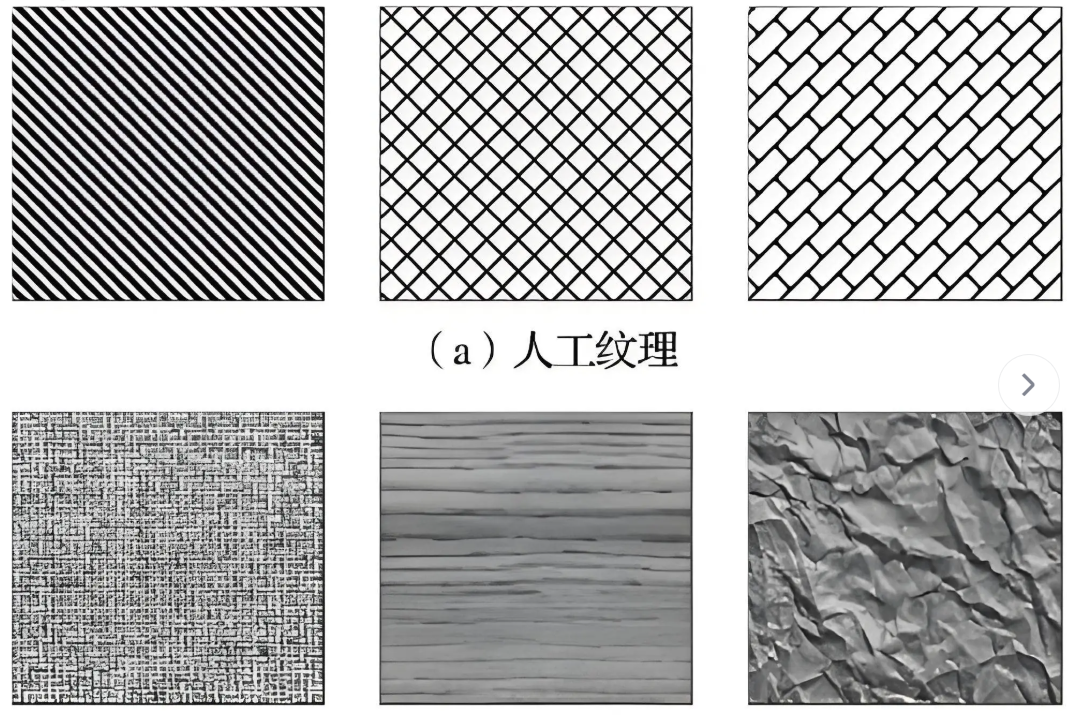

3.1 LBP（局部二值模式）原理与实现

3.1.1 原理

LBP 是最经典的局部纹理特征，核心思想：以中心像素为阈值，将邻域像素的灰度值与中心像素比较，生成二进制编码。公式：\(LBP(x_c,y_c) = \sum_{n=0}^{N-1} s(I_n - I_c)2^n\)其中：\(I_c\)是中心像素灰度，\(I_n\)是邻域像素灰度，\(s(x)\)是符号函数（\(x≥0\)为 1，否则为 0）。

优点：计算速度快、对光照变化鲁棒、适合描述局部纹理。

3.1.2 LBP 代码实现

import numpy as np
import cv2
from skimage.feature import local_binary_pattern

class TextureFeature:
    """传统纹理特征提取工具类：整合LBP、GLCM、HOG"""
    def __init__(self):
        # LBP参数配置
        self.lbp_radius = 3  # LBP邻域半径
        self.lbp_points = 8 * self.lbp_radius  # LBP采样点数量
        self.lbp_method = 'uniform'  # 均匀LBP（减少特征维度）

    def extract_lbp(self, gray_img):
        """
        提取LBP纹理特征
        :param gray_img: 灰度图像 (H,W)
        :return: LBP归一化直方图特征 (一维向量)
        """
        # 计算LBP图像
        lbp_img = local_binary_pattern(gray_img, self.lbp_points, self.lbp_radius, self.lbp_method)
        # 计算LBP直方图（归一化，消除图像尺寸影响）
        hist, _ = np.histogram(lbp_img.ravel(), bins=np.arange(0, self.lbp_points + 3), range=(0, self.lbp_points + 2))
        hist = hist.astype(np.float32)
        hist /= (hist.sum() + 1e-6)  # 归一化
        return hist, lbp_img

3.2 GLCM（灰度共生矩阵）原理与实现

3.2.1 原理

GLCM 通过统计灰度值对在特定方向、距离上的共生频率，提取 4 个核心统计特征：

1. 对比度（Contrast）：描述纹理的清晰程度；
2. 能量（Energy）：描述纹理的均匀程度；
3. 熵（Entropy）：描述纹理的复杂程度；
4. 相关性（Correlation）：描述灰度的线性相关性。

3.2.2 GLCM 代码实现

from skimage.feature import graycomatrix, graycoprops

def extract_glcm(self, gray_img):
    """
    提取GLCM统计纹理特征
    :param gray_img: 灰度图像 (H,W)
    :return: GLCM4维特征向量 [对比度, 能量, 熵, 相关性]
    """
    # 灰度量化为16级（减少计算量）
    gray_quant = (gray_img / 16).astype(np.uint8)
    # 计算GLCM矩阵（方向：0°、45°、90°、135°，距离=1）
    glcm = graycomatrix(gray_quant, distances=[1], angles=[0, np.pi/4, np.pi/2, 3*np.pi/4], levels=16, symmetric=True, normed=True)
    # 提取4个统计特征
    contrast = graycoprops(glcm, 'contrast')[0, 0]
    energy = graycoprops(glcm, 'energy')[0, 0]
    entropy = -np.sum(glcm * np.log2(glcm + 1e-6))  # 手动计算熵
    correlation = graycoprops(glcm, 'correlation')[0, 0]
    # 拼接特征向量
    glcm_feature = np.array([contrast, energy, entropy, correlation], dtype=np.float32)
    return glcm_feature

3.3 HOG（方向梯度直方图）原理与实现

3.3.1 原理

HOG 通过计算图像局部区域的梯度方向直方图，描述目标的边缘与纹理轮廓，适合纹理 + 轮廓的联合表征。

3.3.2 HOG 代码实现

from skimage.feature import hog

def extract_hog(self, gray_img):
    """
    提取HOG梯度纹理特征
    :param gray_img: 灰度图像 (H,W)
    :return: HOG特征向量 (一维向量)
    """
    # 固定图像尺寸（统一特征维度）
    gray_resize = cv2.resize(gray_img, (64, 64))
    # 提取HOG特征
    hog_feature, hog_img = hog(
        gray_resize,
        orientations=9,  # 梯度方向数
        pixels_per_cell=(8, 8),  # 单元格像素数
        cells_per_block=(2, 2),  # 块内单元格数
        block_norm='L2-Hys',  # 归一化方式
        visualize=True,  # 可视化HOG图像
        feature_vector=True
    )
    return hog_feature, hog_img

3.4 纹理特征工具类完整整合

将三个特征整合为统一调用接口，输入 RGB 图像，直接输出融合纹理特征：

import numpy as np
import cv2
from skimage.feature import local_binary_pattern, graycomatrix, graycoprops, hog

class TextureFeature:
    """传统纹理特征提取工具类：LBP + GLCM + HOG"""
    def __init__(self):
        # LBP参数
        self.lbp_radius = 3
        self.lbp_points = 8 * self.lbp_radius
        self.lbp_method = 'uniform'

    def extract_lbp(self, gray_img):
        lbp_img = local_binary_pattern(gray_img, self.lbp_points, self.lbp_radius, self.lbp_method)
        hist, _ = np.histogram(lbp_img.ravel(), bins=np.arange(0, self.lbp_points + 3), range=(0, self.lbp_points + 2))
        hist = hist.astype(np.float32)
        hist /= (hist.sum() + 1e-6)
        return hist, lbp_img

    def extract_glcm(self, gray_img):
        gray_quant = (gray_img / 16).astype(np.uint8)
        glcm = graycomatrix(gray_quant, distances=[1], angles=[0, np.pi/4, np.pi/2, 3*np.pi/4], levels=16, symmetric=True, normed=True)
        contrast = graycoprops(glcm, 'contrast')[0, 0]
        energy = graycoprops(glcm, 'energy')[0, 0]
        entropy = -np.sum(glcm * np.log2(glcm + 1e-6))
        correlation = graycoprops(glcm, 'correlation')[0, 0]
        return np.array([contrast, energy, entropy, correlation], dtype=np.float32)

    def extract_hog(self, gray_img):
        gray_resize = cv2.resize(gray_img, (64, 64))
        hog_feature, hog_img = hog(gray_resize, orientations=9, pixels_per_cell=(8,8), cells_per_block=(2,2), block_norm='L2-Hys', visualize=True, feature_vector=True)
        return hog_feature, hog_img

    def extract_all_texture(self, rgb_img):
        """
        提取融合纹理特征（LBP+GLCM+HOG）
        :param rgb_img: RGB图像 (H,W,3)
        :return: 一维纹理特征向量, 各中间特征图像
        """
        # 转为灰度图
        gray = cv2.cvtColor(rgb_img, cv2.COLOR_RGB2GRAY)
        # 提取单特征
        lbp_feat, lbp_img = self.extract_lbp(gray)
        glcm_feat = self.extract_glcm(gray)
        hog_feat, hog_img = self.extract_hog(gray)
        # 拼接所有纹理特征（归一化后）
        texture_feat = np.concatenate([lbp_feat, glcm_feat, hog_feat])
        return texture_feat, (lbp_img, hog_img, gray)

---

第四章 YOLO11 基础目标检测实现

4.1 YOLO11 模型加载与推理

基于 Ultralytics 库，YOLO11 支持预训练模型直接推理，无需自定义训练，代码极简：

from ultralytics import YOLO
import cv2
import numpy as np

class YOLO11Detector:
    """YOLO11目标检测基础类"""
    def __init__(self, model_path="yolo11n.pt", conf_thres=0.25, iou_thres=0.45):
        """
        初始化YOLO11检测器
        :param model_path: 模型权重（yolo11n/n/s/m/l/x）
        :param conf_thres: 置信度阈值
        :param iou_thres: NMS非极大值抑制阈值
        """
        self.model = YOLO(model_path)
        self.conf_thres = conf_thres
        self.iou_thres = iou_thres
        # 获取COCO类别名称
        self.class_names = self.model.names

    def detect(self, img_path):
        """
        单图像推理
        :param img_path: 图像路径
        :return: 检测结果 [x1,y1,x2,y2,conf,cls_id]
        """
        # 推理（关闭冗余输出）
        results = self.model(img_path, conf=self.conf_thres, iou=self.iou_thres, verbose=False)
        # 解析检测框
        detections = []
        img = cv2.imread(img_path)
        img_rgb = cv2.cvtColor(img, cv2.COLOR_BGR2RGB)
        h, w = img.shape[:2]

        for result in results:
            boxes = result.boxes
            for box in boxes:
                # 提取框坐标、置信度、类别
                x1, y1, x2, y2 = map(int, box.xyxy[0])
                conf = float(box.conf[0])
                cls_id = int(box.cls[0])
                cls_name = self.class_names[cls_id]
                # 保存检测结果
                detections.append({
                    "bbox": [x1, y1, x2, y2],
                    "conf": conf,
                    "cls_id": cls_id,
                    "cls_name": cls_name,
                    "roi": img_rgb[y1:y2, x1:x2]  # 裁剪ROI区域（用于纹理提取）
                })
        return detections, img_rgb

4.2 基础检测测试

创建yolo_base_test.py，测试纯 YOLO11 检测：

if __name__ == "__main__":
    # 初始化检测器
    detector = YOLO11Detector(model_path="yolo11n.pt", conf_thres=0.3)
    # 检测图像（替换为你的图像路径）
    detections, img = detector.detect("test.jpg")
    # 打印结果
    print(f"检测到{len(detections)}个目标：")
    for det in detections:
        print(f"类别：{det['cls_name']}, 置信度：{det['conf']:.2f}, 框：{det['bbox']}")

---

第五章 YOLO11 + 纹理特征融合检测实现

本章节实现两种融合方案，方案 1 为轻量级落地版本，方案 2 为进阶高精度版本。

5.1 方案 1：后处理校验融合（核心代码）

5.1.1 融合逻辑

1. YOLO11 检测出所有目标框；
2. 对每个目标的 ROI 区域提取融合纹理特征；
3. 定义纹理校验规则（针对具体目标，如：猫的 LBP 熵 > 0.5，汽车的 GLCM 对比度 > 10）；
4. 过滤不满足纹理规则的误检框；
5. 输出最终检测结果。

5.1.2 完整融合代码

import cv2
import numpy as np
import matplotlib.pyplot as plt
from yolo11_detector import YOLO11Detector  # 导入YOLO11类
from texture_feature import TextureFeature  # 导入纹理特征类

class YOLO11TextureFusion:
    """YOLO11+传统纹理特征 后处理融合检测器"""
    def __init__(self, yolo_model="yolo11n.pt", conf_thres=0.3):
        # 初始化YOLO11检测器
        self.yolo = YOLO11Detector(model_path=yolo_model, conf_thres=conf_thres)
        # 初始化纹理特征提取器
        self.texture = TextureFeature()
        # 定义纹理校验规则（可根据你的目标自定义！）
        self.texture_rules = {
            # 规则：类别名称 → [最小熵, 最小对比度, 最小能量]
            "cat": [0.5, 8.0, 0.1],
            "dog": [0.4, 6.0, 0.08],
            "car": [0.3, 10.0, 0.12],
            "person": [0.6, 5.0, 0.09]
        }

    def check_texture_valid(self, roi_img, cls_name):
        """
        纹理特征校验：判断目标是否符合纹理规则
        :param roi_img: 目标ROI图像
        :param cls_name: YOLO检测的类别名称
        :return: True=有效目标, False=误检
        """
        try:
            # 提取纹理特征
            texture_feat, (lbp_img, hog_img, gray) = self.texture.extract_all_texture(roi_img)
            # 提取GLCM特征（索引24:28：LBP24维 + GLCM4维）
            contrast, energy, entropy, correlation = texture_feat[24:28]
            # 获取对应类别的纹理规则
            if cls_name not in self.texture_rules:
                return True  # 无规则则默认有效
            min_entropy, min_contrast, min_energy = self.texture_rules[cls_name]
            # 校验规则：纹理特征满足阈值则为有效目标
            if entropy >= min_entropy and contrast >= min_contrast and energy >= min_energy:
                return True
            return False
        except:
            return True  # 异常则默认有效

    def fusion_detect(self, img_path, save_result=True):
        """
        融合检测主函数
        :param img_path: 图像路径
        :param save_result: 是否保存可视化结果
        :return: 最终有效检测结果
        """
        # 1. YOLO11基础检测
        detections, img_rgb = self.yolo.detect(img_path)
        # 2. 纹理特征校验，过滤误检
        valid_detections = []
        for det in detections:
            roi = det["roi"]
            cls_name = det["cls_name"]
            # 纹理校验
            if self.check_texture_valid(roi, cls_name):
                valid_detections.append(det)
        # 3. 可视化结果
        result_img = self.visualize(img_rgb, valid_detections)
        if save_result:
            plt.imsave("fusion_result.jpg", result_img)
            cv2.imwrite("fusion_result_bgr.jpg", cv2.cvtColor(result_img, cv2.COLOR_RGB2BGR))
        # 4. 输出结果
        print(f"YOLO原始检测：{len(detections)}个 | 纹理校验后：{len(valid_detections)}个")
        return valid_detections, result_img

    def visualize(self, img_rgb, detections):
        """可视化检测结果"""
        img = img_rgb.copy()
        for det in detections:
            x1, y1, x2, y2 = det["bbox"]
            cls_name = det["cls_name"]
            conf = det["conf"]
            # 绘制框
            cv2.rectangle(img, (x1, y1), (x2, y2), (0, 255, 0), 2)
            # 绘制类别+置信度
            label = f"{cls_name} {conf:.2f}"
            cv2.putText(img, label, (x1, y1-10), cv2.FONT_HERSHEY_SIMPLEX, 0.5, (0, 255, 0), 2)
        return img

5.1.3 方案 1 测试

创建fusion_test.py，运行融合检测：

if __name__ == "__main__":
    # 初始化融合检测器
    fusion_detector = YOLO11TextureFusion(yolo_model="yolo11n.pt", conf_thres=0.3)
    # 执行融合检测（替换为你的图像路径）
    valid_dets, result_img = fusion_detector.fusion_detect("test.jpg")
    # 打印有效目标
    for det in valid_dets:
        print(f"有效目标：{det['cls_name']}, 置信度：{det['conf']:.2f}")
    # 显示结果
    plt.figure(figsize=(10, 6))
    plt.imshow(result_img)
    plt.axis("off")
    plt.title("YOLO11+纹理特征融合检测结果")
    plt.show()

5.2 方案 2：特征层融合（进阶，高精度）

5.2.1 融合逻辑

修改 YOLO11 的 PAN Neck 网络，将传统纹理特征映射为特征图 ，与 YOLO11 的深层语义特征拼接融合，再输入检测头进行推理，实现端到端的特征融合。

5.2.2 核心修改代码

基于 Ultralytics 源码，修改ultralytics/nn/modules/head.py，添加纹理特征融合层：

# 新增：纹理特征映射层
class TextureFusionBlock(nn.Module):
    def __init__(self, in_channels=1, out_channels=256):
        super().__init__()
        self.conv = nn.Conv2d(in_channels, out_channels, kernel_size=1, stride=1, padding=0)
        self.bn = nn.BatchNorm2d(out_channels)
        self.act = nn.SiLU()

    def forward(self, texture_feat):
        return self.act(self.bn(self.conv(texture_feat)))

# 修改YOLO11的Detect头部，添加纹理特征拼接
class Detect(nn.Module):
    def __init__(self, nc=80, ch=()):
        super().__init__()
        self.nc = nc
        self.reg_max = 16
        self.no = nc + self.reg_max * 4
        # 纹理融合模块
        self.texture_fusion = TextureFusionBlock(in_channels=1, out_channels=ch[0])
        # 原有检测头代码...

    def forward(self, x, texture_map=None):
        # 特征层融合：拼接纹理特征图与YOLO特征图
        if texture_map is not None and self.training:
            texture_feat = self.texture_fusion(texture_map)
            for i in range(len(x)):
                x[i] = torch.cat([x[i], texture_feat], dim=1)
        # 原有推理代码...
        return x