生成对抗网络 GAN:生成模型的经典入门解读
原文:Dive into Deep Learning classic 0.17.6, "Generative Adversarial Networks"
作者:Aston Zhang, Zachary C. Lipton, Mu Li, Alexander J. Smola
原文链接:https://classic.d2l.ai/chapter_generative-adversarial-networks/gan.html
页面版本信息:HTTP Last-Modified 为 2022-11-13;D2L classic 0.17.6
许可说明:D2L 英文仓库 README 的 License Summary 声明,开源书籍文本采用 Creative Commons Attribution-ShareAlike 4.0 International License;示例/参考代码采用修改版 MIT 许可。本文为中文翻译,保留原文结构、公式、代码与图示语义,并按 CC BY-SA 4.0 要求注明来源与许可。
17.1. 生成对抗网络
在本书的大部分篇幅中,我们一直在讨论如何进行预测。无论形式如何,我们使用深度神经网络从数据样本到标签中学习映射。这类学习称为判别式学习。比如,我们希望能够区分猫的照片和狗的照片。分类器和回归器都是判别式学习的例子。通过反向传播训练的神经网络,已经彻底改变了我们过去对大型复杂数据集上判别式学习的认识。短短 5-6 年里,高分辨率图像分类准确率就从几乎不可用提升到了接近人类水平,当然其中仍有一些限制。对于深度神经网络在其他判别式任务上表现优异的例子,这里就不再重复展开。
不过,机器学习并不只是解决判别式任务。比如,给定一个没有任何标签的大型数据集,我们可能希望学习一个模型,用简洁的方式捕捉这些数据的特征。有了这样的模型之后,我们就可以采样出一些合成数据样本,使它们类似于训练数据的分布。举例来说,给定一个庞大的人脸照片语料库,我们也许希望生成一张新的、逼真的人脸图像,让它看起来好像也可能来自同一个数据集。这类学习称为生成式建模。
直到不久以前,我们还没有方法能够合成新的、逼真的照片级图像。但深度神经网络在判别式学习上的成功打开了新的可能性。过去三年里的一个重要趋势,是把判别式深度网络应用到一些通常并不被看作监督学习的问题中,以克服其中的挑战。循环神经网络语言模型就是一个例子:它使用一个判别式网络训练预测下一个字符,而一旦训练完成,它就可以作为生成式模型使用。
2014 年,一篇突破性的论文引入了生成对抗网络(Generative Adversarial Networks, GANs),这是一种巧妙的新方法:借助判别式模型的能力,得到良好的生成式模型。GAN 的核心思想是,如果我们无法把假数据和真实数据区分开,那么这个数据生成器就是好的。在统计学中,这叫做双样本检验,也就是回答这样一个问题:数据集 (X={x_1,\ldots, x_n}) 和 (X'={x'_1,\ldots, x'_n}) 是否来自同一个分布。
大多数统计论文与 GAN 的主要区别在于,后者以一种建设性的方式使用这个思想。换句话说,GAN 并不只是训练一个模型说:"嘿,这两个数据集看起来不像来自同一个分布。"相反,它使用这个双样本检验,为生成式模型提供训练信号。这使我们能够不断改进数据生成器,直到它生成的内容看起来像真实数据。至少,它需要骗过分类器,即使这个分类器是当前最先进的深度神经网络。
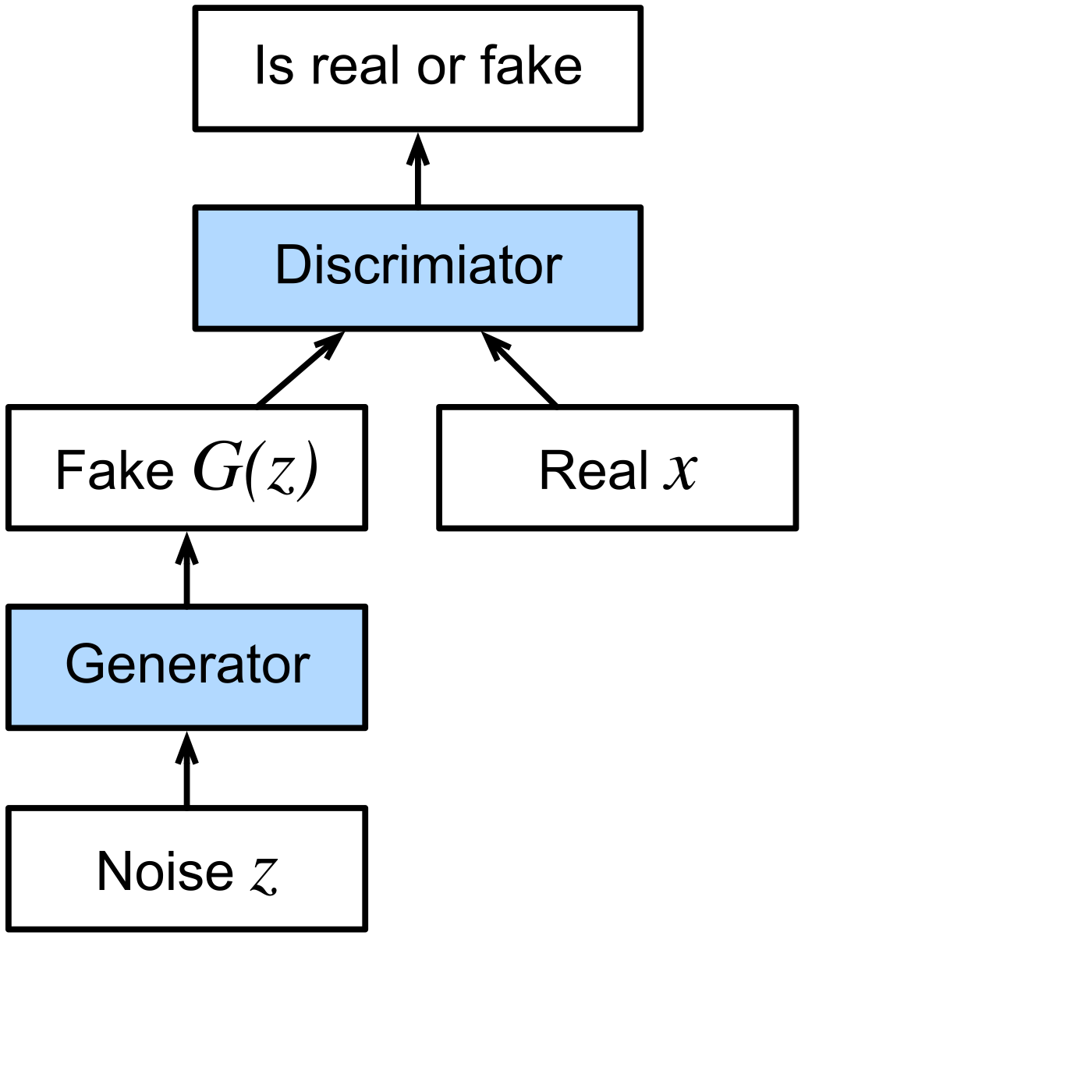
图 17.1.1 展示了 GAN 的架构。可以看到,GAN 架构包含两个部分。首先,我们需要一个设备,比如深度网络,不过它其实可以是任何东西,例如游戏渲染引擎,只要它有可能生成看起来像真实数据的数据即可。如果处理的是图像,它就需要生成图像;如果处理的是语音,它就需要生成音频序列,依此类推。我们称它为生成器网络。
第二个组件是判别器网络。它试图区分假数据和真实数据。这两个网络彼此竞争。生成器网络试图欺骗判别器网络;随后,判别器网络会适应新的假数据;这些信息反过来又被用来改进生成器网络,如此循环。
判别器是一个二分类器,用来判断输入 (x) 是真实的(来自真实数据)还是伪造的(来自生成器)。通常,判别器会对输入 (\mathbf x) 输出一个标量预测 (o\in\mathbb R),例如使用隐藏大小为 1 的全连接层;然后应用 sigmoid 函数得到预测概率:
D(\\mathbf x) = 1/(1+e\^{-o}).
假设真实数据的标签 (y) 为 (1),伪造数据的标签为 (0)。我们训练判别器来最小化交叉熵损失,即:
(17.1.1)
\\min_D { - y \\log D(\\mathbf x) - (1-y)\\log(1-D(\\mathbf x)) },
对于生成器,它首先从某个随机源中抽取参数 (\mathbf z\in\mathbb R^d),例如正态分布 (\mathbf z \sim \mathcal{N} (0, 1))。我们通常把 (\mathbf z) 称为潜变量。随后,它应用一个函数来生成 (\mathbf x'=G(\mathbf z))。生成器的目标是欺骗判别器,让判别器把 (\mathbf x'=G(\mathbf z)) 分类为真实数据,也就是我们希望 (D( G(\mathbf z)) \approx 1)。换句话说,对于给定的判别器 (D),我们更新生成器 (G) 的参数,使得当 (y=0) 时交叉熵损失最大化,即:
(17.1.2)
\\max_G { - (1-y) \\log(1-D(G(\\mathbf z))) } = \\max_G { - \\log(1-D(G(\\mathbf z))) }.
如果生成器做得非常好,那么 (D(\mathbf x')\approx 1),上面的损失就接近 0,这会导致梯度太小,判别器难以取得良好进展。因此,通常我们会最小化下面的损失:
(17.1.3)
\\min_G { - y \\log(D(G(\\mathbf z))) } = \\min_G { - \\log(D(G(\\mathbf z))) },
这相当于把 (\mathbf x'=G(\mathbf z)) 输入判别器,但给它的标签是 (y=1)。
概括来说,(D) 和 (G) 正在进行一个"极小极大"博弈,其综合目标函数为:
(17.1.4)
min_D max_G { -E_{x \\sim \\text{Data}} log D(\\mathbf x) - E_{z \\sim \\text{Noise}} log(1 - D(G(\\mathbf z))) }.
GAN 的许多应用都发生在图像场景中。作为演示,我们先满足于拟合一个简单得多的分布。我们将展示,如果用 GAN 来构建世界上最低效的高斯参数估计器,会发生什么。现在开始。
MXNet
python
%matplotlib inline
from mxnet import autograd, gluon, init, np, npx
from mxnet.gluon import nn
from d2l import mxnet as d2l

npx.set_np()
PyTorch
python
%matplotlib inline
import torch
from torch import nn
from d2l import torch as d2l
TensorFlow
python
import tensorflow as tf
from d2l import tensorflow as d2l
17.1.1. 生成一些"真实"数据
因为这将是世界上最朴素的例子,我们只生成从高斯分布中抽样得到的数据。
MXNet
python
X = np.random.normal(0.0, 1, (1000, 2))
A = np.array([[1, 2], [-0.1, 0.5]])
b = np.array([1, 2])
data = np.dot(X, A) + b
PyTorch
python
X = torch.normal(0.0, 1, (1000, 2))
A = torch.tensor([[1, 2], [-0.1, 0.5]])
b = torch.tensor([1, 2])
data = torch.matmul(X, A) + b
TensorFlow
python
X = tf.random.normal((1000, 2), 0.0, 1)
A = tf.constant([[1, 2], [-0.1, 0.5]])
b = tf.constant([1, 2], tf.float32)
data = tf.matmul(X, A) + b
让我们看看得到了什么。这应该是一个以某种相当任意的方式平移过的高斯分布,其均值为 (b),协方差矩阵为 (A^TA)。
MXNet
python
d2l.set_figsize()
d2l.plt.scatter(data[:100, 0].asnumpy(), data[:100, 1].asnumpy());
print(f'The covariance matrix is\n{np.dot(A.T, A)}')
text
The covariance matrix is
[[1.01 1.95]
 [1.95 4.25]]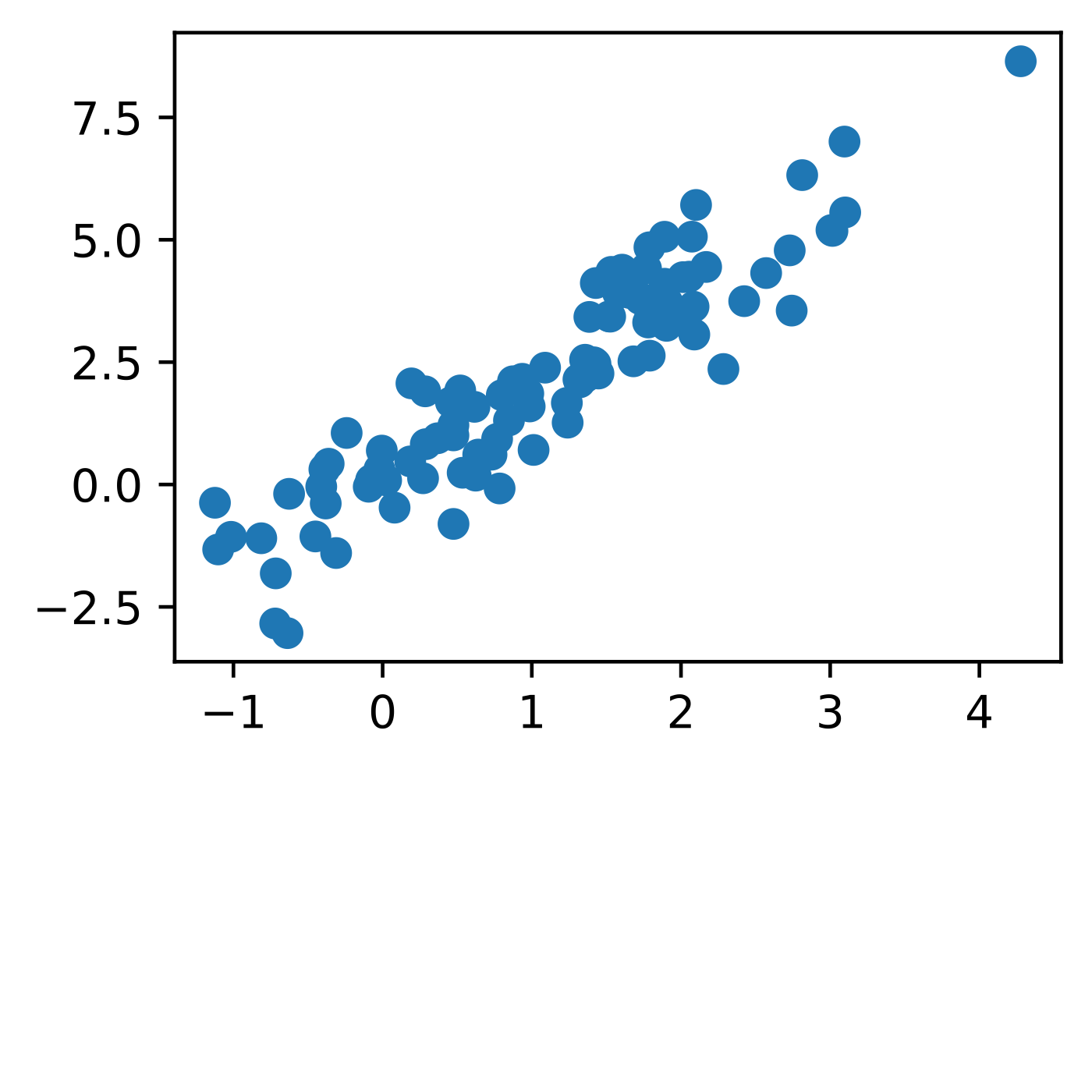
python
batch_size = 8
data_iter = d2l.load_array((data,), batch_size)
PyTorch
python
d2l.set_figsize()
d2l.plt.scatter(data[:100, 0].detach().numpy(), data[:100, 1].detach().numpy());
print(f'The covariance matrix is\n{torch.matmul(A.T, A)}')
text
The covariance matrix is
tensor([[1.0100, 1.9500],
        [1.9500, 4.2500]])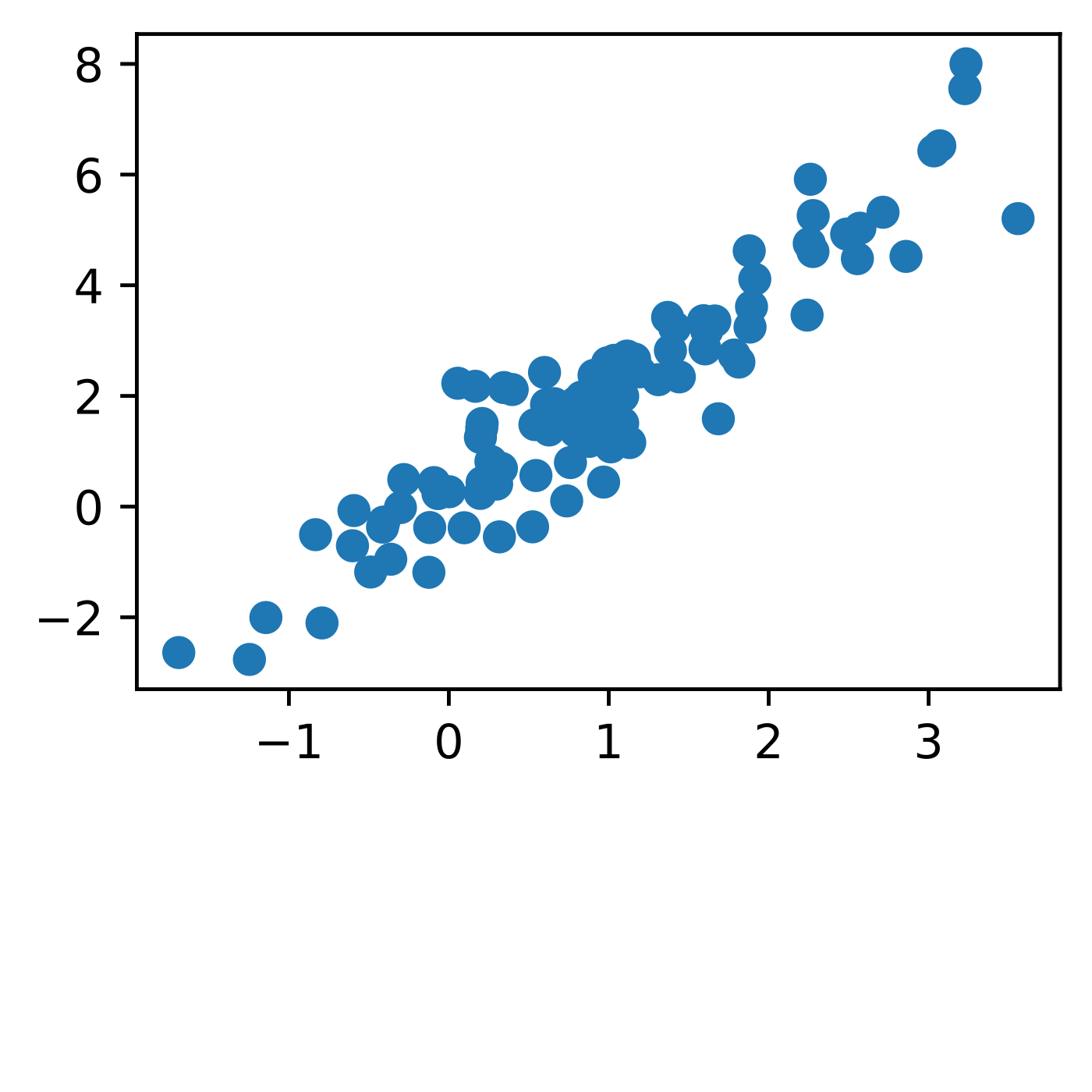
python
batch_size = 8
data_iter = d2l.load_array((data,), batch_size)
TensorFlow
python
d2l.set_figsize()
d2l.plt.scatter(data[:100, 0].numpy(), data[:100, 1].numpy());
print(f'The covariance matrix is\n{tf.matmul(A, A, transpose_a=True)}')
text
The covariance matrix is
[[1.01 1.95]
 [1.95 4.25]]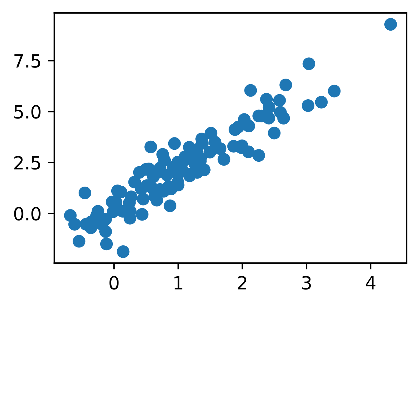
python
batch_size = 8
data_iter = d2l.load_array((data,), batch_size)
17.1.2. 生成器
我们的生成器网络将是尽可能简单的网络:一个单层线性模型。这是因为我们会用一个高斯数据生成器来驱动这个线性网络。因此,从字面上说,它只需要学会一些参数,就可以把数据伪造得足够完美。
MXNet
python
net_G = nn.Sequential()
net_G.add(nn.Dense(2))
PyTorch
python
net_G = nn.Sequential(nn.Linear(2, 2))TensorFlow
python
net_G = tf.keras.layers.Dense(2)17.1.3. 判别器
对于判别器,我们会稍微更有辨别能力一些:它将是一个包含 3 层的多层感知机,让事情稍微变得有趣一点。
MXNet
python
net_D = nn.Sequential()
net_D.add(nn.Dense(5, activation='tanh'),
          nn.Dense(3, activation='tanh'),
          nn.Dense(1))
PyTorch
python
net_D = nn.Sequential(
    nn.Linear(2, 5), nn.Tanh(),
    nn.Linear(5, 3), nn.Tanh(),
    nn.Linear(3, 1))
TensorFlow
python
net_D = tf.keras.models.Sequential([
    tf.keras.layers.Dense(5, activation="tanh", input_shape=(2,)),
    tf.keras.layers.Dense(3, activation="tanh"),
    tf.keras.layers.Dense(1)
])
17.1.4. 训练
首先,我们定义一个函数来更新判别器。
MXNet
python
#@save
def update_D(X, Z, net_D, net_G, loss, trainer_D):
    """Update discriminator."""
    batch_size = X.shape[0]
    ones = np.ones((batch_size,), ctx=X.ctx)
    zeros = np.zeros((batch_size,), ctx=X.ctx)
    with autograd.record():
        real_Y = net_D(X)
        fake_X = net_G(Z)
        # Do not need to compute gradient for `net_G`, detach it from
        # computing gradients.
        fake_Y = net_D(fake_X.detach())
        loss_D = (loss(real_Y, ones) + loss(fake_Y, zeros)) / 2
    loss_D.backward()
    trainer_D.step(batch_size)
    return float(loss_D.sum())
PyTorch
python
#@save
def update_D(X, Z, net_D, net_G, loss, trainer_D):
    """Update discriminator."""
    batch_size = X.shape[0]
    ones = torch.ones((batch_size,), device=X.device)
    zeros = torch.zeros((batch_size,), device=X.device)
    trainer_D.zero_grad()
    real_Y = net_D(X)
    fake_X = net_G(Z)
    # Do not need to compute gradient for `net_G`, detach it from
    # computing gradients.
    fake_Y = net_D(fake_X.detach())
    loss_D = (loss(real_Y, ones.reshape(real_Y.shape)) +
              loss(fake_Y, zeros.reshape(fake_Y.shape))) / 2
    loss_D.backward()
    trainer_D.step()
    return loss_D
TensorFlow
python
#@save
def update_D(X, Z, net_D, net_G, loss, optimizer_D):
    """Update discriminator."""
    batch_size = X.shape[0]
    ones = tf.ones((batch_size,)) # Labels corresponding to real data
    zeros = tf.zeros((batch_size,)) # Labels corresponding to fake data
    # Do not need to compute gradient for `net_G`, so it's outside GradientTape
    fake_X = net_G(Z)
    with tf.GradientTape() as tape:
        real_Y = net_D(X)
        fake_Y = net_D(fake_X)
        # We multiply the loss by batch_size to match PyTorch's BCEWithLogitsLoss
        loss_D = (loss(ones, tf.squeeze(real_Y)) + loss(
            zeros, tf.squeeze(fake_Y))) * batch_size / 2
    grads_D = tape.gradient(loss_D, net_D.trainable_variables)
    optimizer_D.apply_gradients(zip(grads_D, net_D.trainable_variables))
    return loss_D
生成器的更新与此类似。这里我们复用交叉熵损失,但把生成样本的标签设为真实,也就是 (1)。
MXNet
python
#@save
def update_G(Z, net_D, net_G, loss, trainer_G):
    """Update generator."""
    batch_size = Z.shape[0]
    ones = np.ones((batch_size,), ctx=Z.ctx)
    with autograd.record():
        # We could reuse `fake_X` from `update_D` to save computation
        fake_X = net_G(Z)
        # Recomputing `fake_Y` is needed since `net_D` is changed
        fake_Y = net_D(fake_X)
        loss_G = loss(fake_Y, ones)
    loss_G.backward()
    trainer_G.step(batch_size)
    return float(loss_G.sum())
PyTorch
python
#@save
def update_G(Z, net_D, net_G, loss, trainer_G):
    """Update generator."""
    batch_size = Z.shape[0]
    ones = torch.ones((batch_size,), device=Z.device)
    trainer_G.zero_grad()
    # We could reuse `fake_X` from `update_D` to save computation
    fake_X = net_G(Z)
    # Recomputing `fake_Y` is needed since `net_D` is changed
    fake_Y = net_D(fake_X)
    loss_G = loss(fake_Y, ones.reshape(fake_Y.shape))
    loss_G.backward()
    trainer_G.step()
    return loss_G
TensorFlow
python
#@save
def update_G(Z, net_D, net_G, loss, optimizer_G):
    """Update generator."""
    batch_size = Z.shape[0]
    ones = tf.ones((batch_size,))
    with tf.GradientTape() as tape:
        # We could reuse `fake_X` from `update_D` to save computation
        fake_X = net_G(Z)
        # Recomputing `fake_Y` is needed since `net_D` is changed
        fake_Y = net_D(fake_X)
        # We multiply the loss by batch_size to match PyTorch's BCEWithLogits loss
        loss_G = loss(ones, tf.squeeze(fake_Y)) * batch_size
    grads_G = tape.gradient(loss_G, net_G.trainable_variables)
    optimizer_G.apply_gradients(zip(grads_G, net_G.trainable_variables))
    return loss_G
判别器和生成器都会使用交叉熵损失执行二元逻辑回归。我们使用 Adam 来平滑训练过程。在每一次迭代中,我们先更新判别器,然后更新生成器。我们会同时可视化两个损失以及生成出来的样本。
MXNet
python
def train(net_D, net_G, data_iter, num_epochs, lr_D, lr_G, latent_dim, data):
    loss = gluon.loss.SigmoidBCELoss()
    net_D.initialize(init=init.Normal(0.02), force_reinit=True)
    net_G.initialize(init=init.Normal(0.02), force_reinit=True)
    trainer_D = gluon.Trainer(net_D.collect_params(),
                              'adam', {'learning_rate': lr_D})
    trainer_G = gluon.Trainer(net_G.collect_params(),
                              'adam', {'learning_rate': lr_G})
    animator = d2l.Animator(xlabel='epoch', ylabel='loss',
                            xlim=[1, num_epochs], nrows=2, figsize=(5, 5),
                            legend=['discriminator', 'generator'])
    animator.fig.subplots_adjust(hspace=0.3)
    for epoch in range(num_epochs):
        # Train one epoch
        timer = d2l.Timer()
        metric = d2l.Accumulator(3)  # loss_D, loss_G, num_examples
        for X in data_iter:
            batch_size = X.shape[0]
            Z = np.random.normal(0, 1, size=(batch_size, latent_dim))
            metric.add(update_D(X, Z, net_D, net_G, loss, trainer_D),
                       update_G(Z, net_D, net_G, loss, trainer_G),
                       batch_size)
        # Visualize generated examples
        Z = np.random.normal(0, 1, size=(100, latent_dim))
        fake_X = net_G(Z).asnumpy()
        animator.axes[1].cla()
        animator.axes[1].scatter(data[:, 0], data[:, 1])
        animator.axes[1].scatter(fake_X[:, 0], fake_X[:, 1])
        animator.axes[1].legend(['real', 'generated'])
        # Show the losses
        loss_D, loss_G = metric[0]/metric[2], metric[1]/metric[2]
        animator.add(epoch + 1, (loss_D, loss_G))
    print(f'loss_D {loss_D:.3f}, loss_G {loss_G:.3f}, '
          f'{metric[2] / timer.stop():.1f} examples/sec')
PyTorch
python
def train(net_D, net_G, data_iter, num_epochs, lr_D, lr_G, latent_dim, data):
    loss = nn.BCEWithLogitsLoss(reduction='sum')
    for w in net_D.parameters():
        nn.init.normal_(w, 0, 0.02)
    for w in net_G.parameters():
        nn.init.normal_(w, 0, 0.02)
    trainer_D = torch.optim.Adam(net_D.parameters(), lr=lr_D)
    trainer_G = torch.optim.Adam(net_G.parameters(), lr=lr_G)
    animator = d2l.Animator(xlabel='epoch', ylabel='loss',
                            xlim=[1, num_epochs], nrows=2, figsize=(5, 5),
                            legend=['discriminator', 'generator'])
    animator.fig.subplots_adjust(hspace=0.3)
    for epoch in range(num_epochs):
        # Train one epoch
        timer = d2l.Timer()
        metric = d2l.Accumulator(3)  # loss_D, loss_G, num_examples
        for (X,) in data_iter:
            batch_size = X.shape[0]
            Z = torch.normal(0, 1, size=(batch_size, latent_dim))
            metric.add(update_D(X, Z, net_D, net_G, loss, trainer_D),
                       update_G(Z, net_D, net_G, loss, trainer_G),
                       batch_size)
        # Visualize generated examples
        Z = torch.normal(0, 1, size=(100, latent_dim))
        fake_X = net_G(Z).detach().numpy()
        animator.axes[1].cla()
        animator.axes[1].scatter(data[:, 0], data[:, 1])
        animator.axes[1].scatter(fake_X[:, 0], fake_X[:, 1])
        animator.axes[1].legend(['real', 'generated'])
        # Show the losses
        loss_D, loss_G = metric[0]/metric[2], metric[1]/metric[2]
        animator.add(epoch + 1, (loss_D, loss_G))
    print(f'loss_D {loss_D:.3f}, loss_G {loss_G:.3f}, '
          f'{metric[2] / timer.stop():.1f} examples/sec')
TensorFlow
python
def train(net_D, net_G, data_iter, num_epochs, lr_D, lr_G, latent_dim, data):
    loss = tf.keras.losses.BinaryCrossentropy(
        from_logits=True, reduction=tf.keras.losses.Reduction.SUM)
    for w in net_D.trainable_variables:
        w.assign(tf.random.normal(mean=0, stddev=0.02, shape=w.shape))
    for w in net_G.trainable_variables:
        w.assign(tf.random.normal(mean=0, stddev=0.02, shape=w.shape))
    optimizer_D = tf.keras.optimizers.Adam(learning_rate=lr_D)
    optimizer_G = tf.keras.optimizers.Adam(learning_rate=lr_G)
    animator = d2l.Animator(
        xlabel="epoch", ylabel="loss", xlim=[1, num_epochs], nrows=2,
        figsize=(5, 5), legend=["discriminator", "generator"])
    animator.fig.subplots_adjust(hspace=0.3)
    for epoch in range(num_epochs):
        # Train one epoch
        timer = d2l.Timer()
        metric = d2l.Accumulator(3)  # loss_D, loss_G, num_examples
        for (X,) in data_iter:
            batch_size = X.shape[0]
            Z = tf.random.normal(
                mean=0, stddev=1, shape=(batch_size, latent_dim))
            metric.add(update_D(X, Z, net_D, net_G, loss, optimizer_D),
                       update_G(Z, net_D, net_G, loss, optimizer_G),
                       batch_size)
        # Visualize generated examples
        Z = tf.random.normal(mean=0, stddev=1, shape=(100, latent_dim))
        fake_X = net_G(Z)
        animator.axes[1].cla()
        animator.axes[1].scatter(data[:, 0], data[:, 1])
        animator.axes[1].scatter(fake_X[:, 0], fake_X[:, 1])
        animator.axes[1].legend(["real", "generated"])

        # Show the losses
        loss_D, loss_G = metric[0] / metric[2], metric[1] / metric[2]
        animator.add(epoch + 1, (loss_D, loss_G))

    print(f'loss_D {loss_D:.3f}, loss_G {loss_G:.3f}, '
          f'{metric[2] / timer.stop():.1f} examples/sec')
现在,我们指定超参数来拟合这个高斯分布。
MXNet
python
lr_D, lr_G, latent_dim, num_epochs = 0.05, 0.005, 2, 20
train(net_D, net_G, data_iter, num_epochs, lr_D, lr_G,
      latent_dim, data[:100].asnumpy())
text
loss_D 0.693, loss_G 0.693, 319.0 examples/sec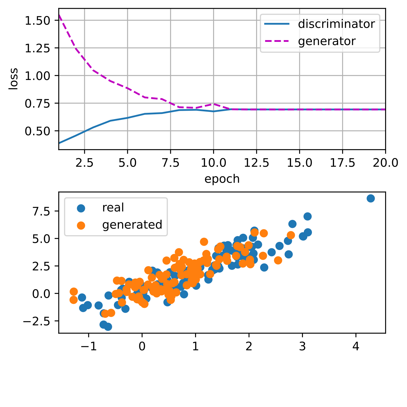
PyTorch
python
lr_D, lr_G, latent_dim, num_epochs = 0.05, 0.005, 2, 20
train(net_D, net_G, data_iter, num_epochs, lr_D, lr_G,
      latent_dim, data[:100].detach().numpy())
text
loss_D 0.693, loss_G 0.693, 1635.3 examples/sec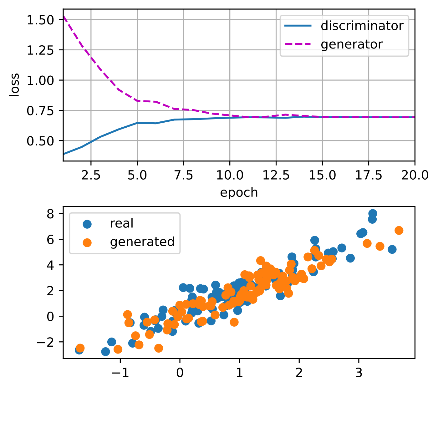
TensorFlow
python
lr_D, lr_G, latent_dim, num_epochs = 0.05, 0.005, 2, 20
train(net_D, net_G, data_iter, num_epochs, lr_D, lr_G,
      latent_dim, data[:100].numpy())
text
loss_D 0.693, loss_G 0.693, 334.8 examples/sec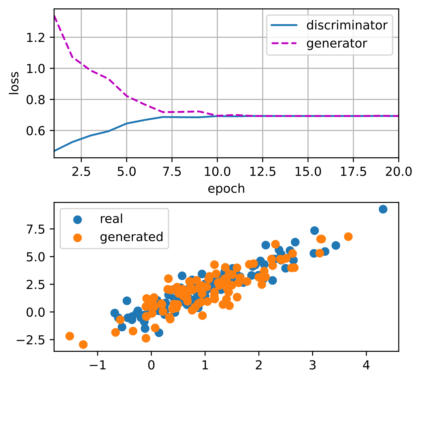
17.1.5. 小结
- 生成对抗网络由两个深度网络组成:生成器和判别器。
- 生成器生成尽可能接近真实图像的图像,使判别器难以区分真假。
- 判别器试图区分真实图像和生成图像。
- 生成器和判别器通过极小极大博弈相互训练。
17.1.6. 练习
- 如果我们把判别器和生成器的学习率改成一样,会发生什么?
- 如果把潜变量的维度从 2 改成 10,会发生什么?
- 你能否证明,方程 (17.1.4) 等价于最小化数据分布和生成器分布之间的 Jensen-Shannon 散度?