【零基础学智能仿真-11】CatBoost——让材料类型和边界条件参与力学预测

课程摘要

本节学习能够直接处理类别特征的CatBoost算法。课程以三种材料和两种支承形式的梁响应预测为案例，讲解类别变量、目标统计、Ordered Boosting及对称树结构，并完成分层划分、模型训练、测试评价和误差诊断。通过实际代码与图表，学习者将认识材料名称、单元类型和边界条件不能随意数字化，掌握混合类型有限元数据的建模方法，同时理解未知类别、数据泄漏和极端工况预测的风险。

课程摘要

本节学习能够直接处理类别特征的CatBoost算法。课程以三种材料和两种支承形式的梁响应预测为案例，讲解类别变量、目标统计、Ordered Boosting及对称树结构，并完成分层划分、模型训练、测试评价和误差诊断。通过实际代码与图表，学习者将认识材料名称、单元类型和边界条件不能随意数字化，掌握混合类型有限元数据的建模方法，同时理解未知类别、数据泄漏和极端工况预测的风险。

---

一、本节学习目标

完成本节后，你将能够：

1. 区分数值特征与类别特征；
2. 理解为什么不能随意给材料类型编号；
3. 理解CatBoost处理类别变量的基本方法；
4. 理解Ordered Boosting解决的核心问题；
5. 使用CatBoostRegressor训练力学响应模型；
6. 对材料与支承组合进行分层数据划分；
7. 使用学习曲线、预测图和残差图评价模型；
8. 正确处理预测阶段出现的新类别。

---

二、力学数据不只有数字

前面几节使用的输入主要是：

• 载荷F；
• 长度L；
• 弹性模量E；
• 截面宽度b；
• 截面高度h。

这些都属于数值特征。

但真实有限元数据还经常包含：

特征	示例	类型
材料类型	钢、铝合金、钛合金	类别特征
支承形式	固定、简支、弹性支承	类别特征
单元类型	C3D8R、C3D10、S4R	类别特征
分析步类型	Static、Dynamic、HeatTransfer	类别特征
接触形式	无摩擦、罚函数、硬接触	类别特征
几何尺寸	长度、厚度、孔径	数值特征
载荷条件	压力、力、温度	数值特征

因此，真实的力学机器学习问题往往是：

\ \\text{数值特征}+\\text{类别特征} \\longrightarrow \\text{力学响应} \\

---

三、为什么不能把类别随意编号？

假设有三种材料：

Steel
Aluminum
Titanium

如果人为编码为：

Steel      = 1
Aluminum   = 2
Titanium   = 3

普通模型可能错误地认为：

\ \\text{Titanium}\>\\text{Aluminum}\>\\text{Steel} \\

甚至认为三个数字之间存在等距关系：

\ 3-2=2-1 \\

但这些编号只是名称，不具有连续数值意义。

同样，如果单元类型被编码为：

C3D8R  = 1
C3D10  = 2
S4R    = 3

数字大小也不代表单元的精度、维度或计算成本。

因此：

\ \\text{类别编号} \\neq \\text{物理量大小} \\

CatBoost的优势之一，就是能够直接接收字符串类别，而不需要学习者提前把材料名称转换成随意的整数。

官方文档也明确提醒，不要在使用CatBoost前盲目进行One-Hot编码，因为这可能影响训练效率和模型效果。CatBoost类别特征说明

---

四、CatBoost怎样处理类别特征？

CatBoost是Categorical Boosting的缩写。它仍然属于梯度提升树，但对类别特征进行了专门设计。

4.1 目标统计编码

假设某个材料类别为"Steel"，一种直观的编码方式是计算该类别对应目标值的平均数：

\ \\operatorname{TS}(\\text{Steel}) = \\frac{ \\sum_{i:x_i=\\text{Steel}}y_i }{ \\sum_{i:x_i=\\text{Steel}}1 } \\

问题在于：如果计算某个样本的类别统计时使用了该样本自己的目标值，就可能造成目标泄漏。

模型会间接"偷看答案"。

4.2 有序目标统计

CatBoost会对训练样本建立一定顺序。对于第i个样本，只使用排在它前面的样本计算类别统计：

\ \\operatorname{TS}_i = \\frac{ \\displaystyle \\sum_{j\

其中：

• \\mathbf{1}(x_j=x_i)表示类别相同时取1；
• P是先验值；
• a控制先验强度；
• 当前样本自己的目标值不参与自己的编码。

这样可以减轻类别编码中的目标泄漏和预测偏移。

CatBoost还能够根据多个类别构造组合特征，例如：

\ \\text{材料类型} + \\text{支承形式} \\

从而识别"某种材料在某种支承条件下"的响应差异。类别特征转换说明

---

五、什么是Ordered Boosting？

普通梯度提升使用当前模型计算所有训练样本的梯度，再训练下一棵树。

如果同一批样本既参与当前预测，又参与梯度估计，可能产生一定的预测偏移。

Ordered Boosting的基本思想是：

对一个样本计算模型状态和梯度时，只使用排列在它前面的训练样本。

可概括为：

\ \\text{样本排列} \\longrightarrow \\text{只看历史样本} \\longrightarrow \\text{计算类别统计} \\longrightarrow \\text{更新提升树} \\

"Ordered"并不是时间序列预测的意思，而是一种用于训练和类别统计计算的数据排列机制。

CatBoost通常还使用对称树：同一层的所有节点采用相同的分裂条件。对称结构便于快速预测和控制模型结构，但并不意味着它天然满足力学对称性。

---

六、实战问题：混合材料与支承形式的梁响应

本节构造一个同时包含数值特征和类别特征的案例。

6.1 材料类别

材料	弹性模量
Steel	210000\\ \\text{MPa}
Aluminum	70000\\ \\text{MPa}
Titanium	110000\\ \\text{MPa}

在模型输入中，我们只保留材料名称，不直接提供弹性模量。模型需要从数据中学习材料类别与刚度的关系。

6.2 支承类别

设置两类梁问题：

悬臂梁自由端集中载荷：

\ u_{\\mathrm{cantilever}} = \\frac{FL\^3}{3EI} \\

简支梁跨中集中载荷：

\ u_{\\mathrm{simply}} = \\frac{FL\^3}{48EI} \\

矩形截面的截面二次矩为：

\ I=\\frac{bh\^3}{12} \\

因此，模型输入为：

\ (F,L,b,h,\\text{material},\\text{support}) \\

模型输出为：

\ u_{\\max} \\

这里的u_{\\max}表示挠度大小：

• 悬臂梁对应自由端挠度；
• 简支梁对应跨中最大挠度。

本节数据来自经典梁公式，不是Abaqus计算结果，也没有添加随机噪声。

---

七、生成混合类型数据集

import numpy as np
import pandas as pd

rng = np.random.default_rng(42)
n = 3000

materials = np.array([
    "Steel",
    "Aluminum",
    "Titanium"
])

supports = np.array([
    "Cantilever",
    "SimplySupported"
])

E_map = {
    "Steel": 210000.0,
    "Aluminum": 70000.0,
    "Titanium": 110000.0
}

coefficient_map = {
    "Cantilever": 1.0 / 3.0,
    "SimplySupported": 1.0 / 48.0
}

data = pd.DataFrame({
    "F_N": rng.uniform(1, 5, n),
    "L_mm": rng.uniform(300, 600, n),
    "b_mm": rng.uniform(15, 30, n),
    "h_mm": rng.uniform(10, 20, n),
    "material": rng.choice(materials, n),
    "support": rng.choice(supports, n)
})

E = data["material"].map(E_map).to_numpy()

coefficient = (
    data["support"]
    .map(coefficient_map)
    .to_numpy()
)

I = (
    data["b_mm"].to_numpy()
    * data["h_mm"].to_numpy() ** 3
    / 12
)

data["u_mm"] = (
    coefficient
    * data["F_N"].to_numpy()
    * data["L_mm"].to_numpy() ** 3
    / (E * I)
)

print(data.head().to_string(index=False))
print("\n样本数量：", len(data))

预期输出形式

由于表格较宽，具体数值会显示为：

     F_N       L_mm      b_mm      h_mm  material          support     u_mm
3.****     4**.****    **.****    **.****  Steel    SimplySupported  0.****
...

样本数量： 3000

由于随机种子固定，完整脚本每次运行都会生成相同数据。

---

八、先观察类别与响应的关系

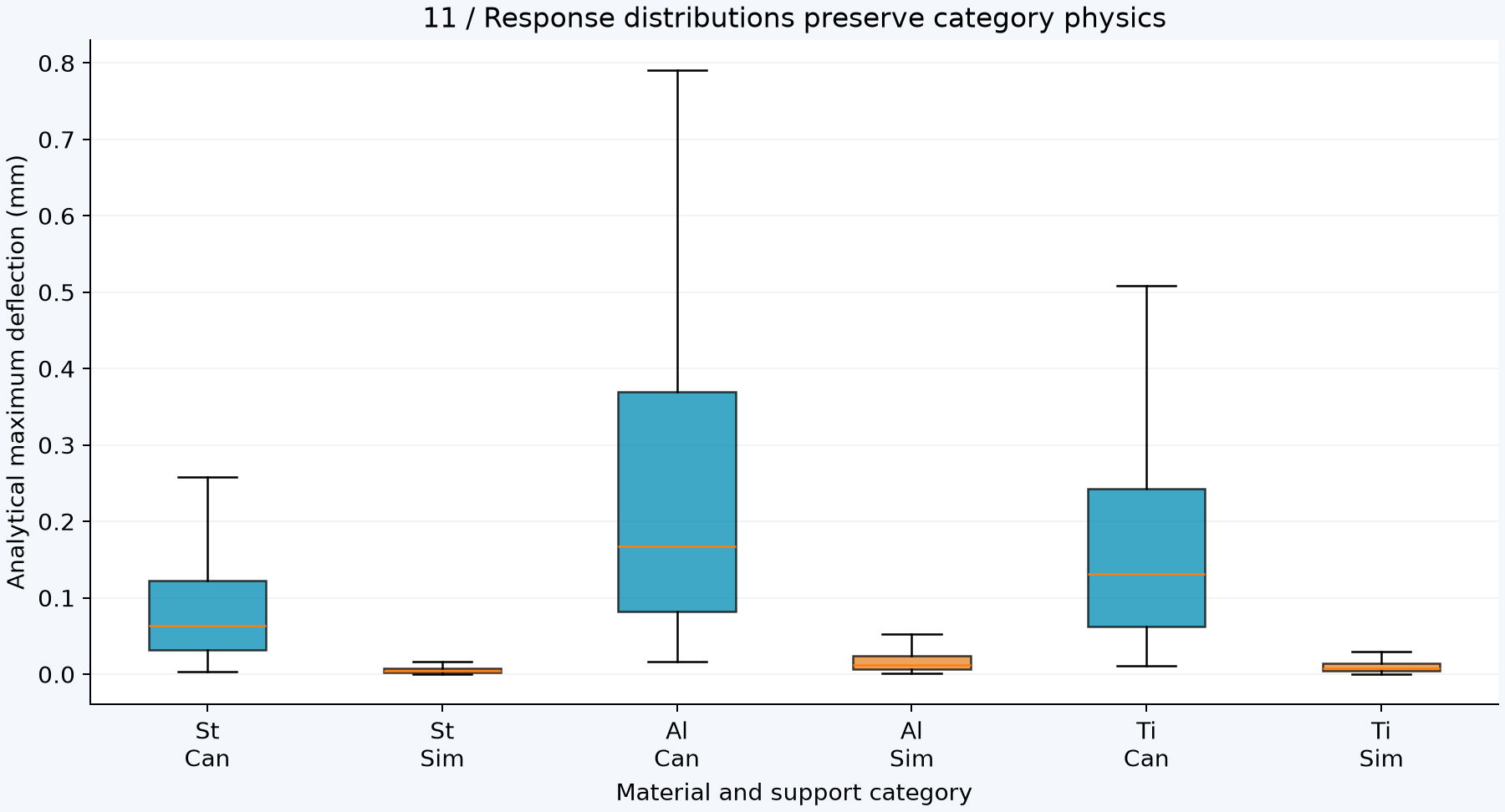
图11-1　不同材料和支承形式的挠度分布

图中的缩写分别表示：

• St：Steel；
• Al：Aluminum；
• Ti：Titanium；
• Can：Cantilever；
• Sim：SimplySupported。

从图中可以看到：

1. 相同材料下，悬臂梁挠度明显大于简支梁；
2. 相同支承条件下，铝合金挠度总体更大；
3. 支承形式对响应分布的影响非常显著；
4. 同一类别中仍存在较大离散，因为F、L、b、h也在变化。

这说明类别变量不是无关的文字标签，而是对力学模型的物理条件描述。

---

九、分层划分训练集、验证集和测试集

本案例共有：

\ 3\\times2=6 \\

种"材料×支承"组合。

如果直接随机划分，理论上可能出现某些小类别在测试集中数量过少。为此，可以按照类别组合进行分层划分。

from sklearn.model_selection import train_test_split

feature_names = [
    "F_N",
    "L_mm",
    "b_mm",
    "h_mm",
    "material",
    "support"
]

category_names = [
    "material",
    "support"
]

index = np.arange(len(data))

strata = (
    data["material"]
    + "|"
    + data["support"]
).to_numpy()

index_dev, index_test = train_test_split(
    index,
    test_size=0.20,
    random_state=42,
    stratify=strata
)

index_train, index_val = train_test_split(
    index_dev,
    test_size=0.25,
    random_state=42,
    stratify=strata[index_dev]
)

X_train = data.loc[index_train, feature_names]
y_train = data.loc[index_train, "u_mm"]

X_val = data.loc[index_val, feature_names]
y_val = data.loc[index_val, "u_mm"]

X_test = data.loc[index_test, feature_names]
y_test = data.loc[index_test, "u_mm"]

print("训练集：", len(y_train))
print("验证集：", len(y_val))
print("测试集：", len(y_test))

预期输出

训练集： 1800
验证集： 600
测试集： 600

完整代码还会检查测试集中的类别组合：

Test category combinations: 6 / 6
min count=93

说明6种组合都进入了测试集，每种组合至少有93个测试样本。

---

十、建立CatBoost数据池

CatBoost可以直接接收Pandas表格，也可以使用Pool明确指定数据和类别列。

from catboost import Pool

train_pool = Pool(
    data=X_train,
    label=y_train,
    cat_features=category_names
)

val_pool = Pool(
    data=X_val,
    label=y_val,
    cat_features=category_names
)

test_pool = Pool(
    data=X_test,
    label=y_test,
    cat_features=category_names
)

这里最重要的是：

cat_features=category_names

它告诉CatBoost：

material和support是类别，不是普通字符串错误，也不是连续数值。

如果使用特征名称指定类别列，输入数据应保留列名，例如使用Pandas DataFrame。官方接口支持通过列名或列索引指定类别特征。CatBoostRegressor接口

---

十一、训练CatBoost回归模型

首先安装依赖：

python -m pip install numpy pandas scikit-learn matplotlib catboost

建立模型：

from catboost import CatBoostRegressor

model = CatBoostRegressor(
    loss_function="RMSE",
    eval_metric="RMSE",

    iterations=3000,
    learning_rate=0.03,
    depth=6,

    l2_leaf_reg=5.0,
    random_strength=0.5,

    boosting_type="Ordered",

    bootstrap_type="Bernoulli",
    subsample=0.85,

    random_seed=42,
    thread_count=2,

    allow_writing_files=False,
    verbose=False
)

参数解释

参数	作用
iterations	最大提升轮数
learning_rate	每棵树的更新幅度
depth	对称树深度
l2_leaf_reg	叶节点输出的L2正则化
random_strength	分裂选择中的随机扰动
boosting_type	本节显式选择Ordered Boosting
bootstrap_type	样本重采样方法
subsample	每轮使用的训练样本比例
thread_count	CPU训练线程数
allow_writing_files	是否创建默认训练日志文件

开始训练：

import time

start = time.perf_counter()

model.fit(
    train_pool,
    eval_set=val_pool,
    early_stopping_rounds=100,
    use_best_model=True,
    verbose=False
)

elapsed = time.perf_counter() - start

history = model.get_evals_result()

print(
    "最佳迭代轮数：",
    model.get_best_iteration() + 1
)

print(
    "模型保留树数量：",
    model.tree_count_
)

print(
    "实际评估轮数：",
    len(history["learn"]["RMSE"])
)

print(f"本机训练耗时：{elapsed:.4f} s")

本次实际输出

最佳迭代轮数： 2997
模型保留树数量： 2997
实际评估轮数： 3000
本机训练耗时：146.1888 s

为什么早停没有提前终止？

本次最优结果出现在第2997轮，而最大轮数是3000。训练完成前，没有出现连续100轮不改善的情况，因此早停没有真正触发。

但由于：

use_best_model=True

最终仍只保留验证指标最好的2997棵树。

这说明：

\ \\text{设置了早停} \\neq \\text{一定会提前停止} \\

训练耗时与CPU、软件版本和后台负载有关，146秒只是本机实测结果。

---

十二、绘制学习曲线

import matplotlib.pyplot as plt

rounds = np.arange(
    1,
    len(history["learn"]["RMSE"]) + 1
)

plt.plot(
    rounds,
    history["learn"]["RMSE"],
    label="Training"
)

plt.plot(
    rounds,
    history["validation"]["RMSE"],
    label="Validation"
)

plt.axvline(
    model.get_best_iteration() + 1,
    color="black",
    linestyle="--",
    label="Best round"
)

plt.xlabel("Boosting round")
plt.ylabel("RMSE (mm)")
plt.legend()
plt.grid(alpha=0.3)
plt.tight_layout()
plt.show()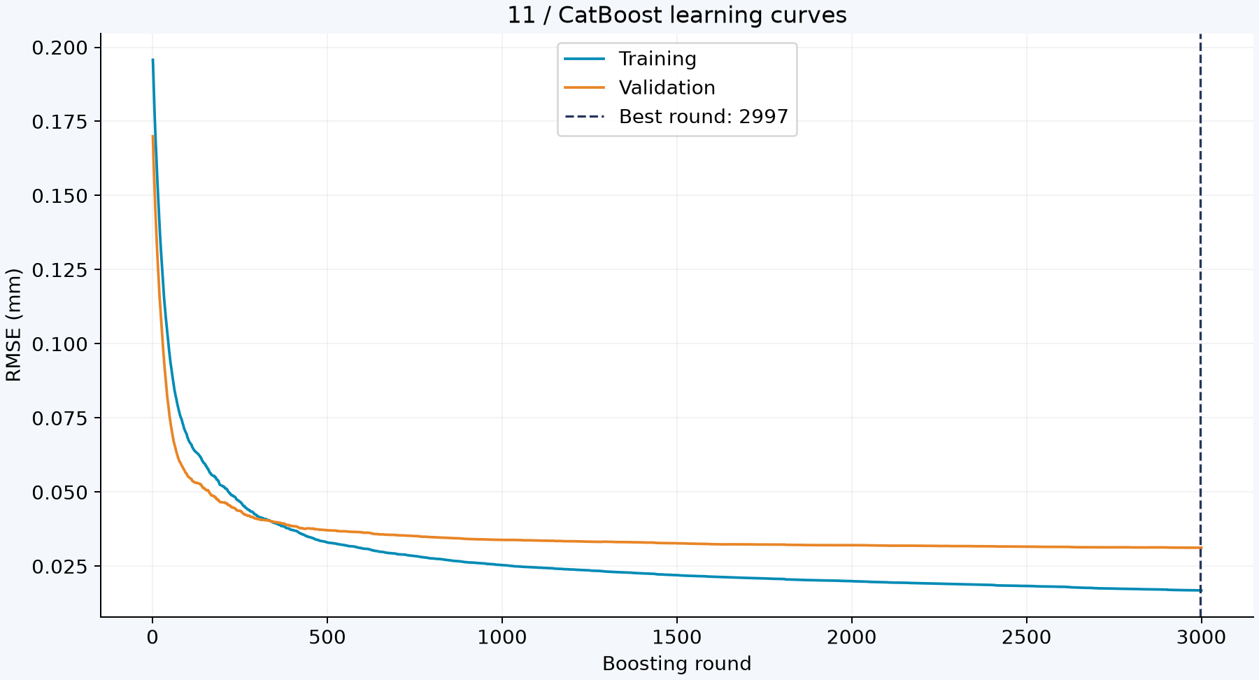

图11-2　CatBoost学习曲线

可以看到：

• 训练初期误差快速下降；
• 后期训练误差继续下降；
• 验证误差改善越来越缓慢；
• 最佳点出现在训练上限附近。

这提示我们：如果继续追求更高精度，应先改善数据覆盖和物理特征，而不是简单无限增加迭代轮数。

---

十三、评价测试集预测结果

from sklearn.metrics import (
    mean_absolute_error,
    mean_squared_error,
    r2_score
)

y_pred = model.predict(test_pool)

baseline = np.full(
    len(y_test),
    y_train.mean()
)

baseline_rmse = np.sqrt(
    mean_squared_error(y_test, baseline)
)

rmse = np.sqrt(
    mean_squared_error(y_test, y_pred)
)

mae = mean_absolute_error(
    y_test,
    y_pred
)

r2 = r2_score(
    y_test,
    y_pred
)

print(f"Baseline RMSE: {baseline_rmse:.6f} mm")
print(f"CatBoost RMSE: {rmse:.6f} mm")
print(f"CatBoost MAE: {mae:.6f} mm")
print(f"CatBoost R2: {r2:.6f}")

本次实际输出

Baseline RMSE: 0.179774 mm
CatBoost RMSE: 0.030647 mm
CatBoost MAE: 0.012084 mm
CatBoost R2: 0.970925

模型明显优于"始终预测训练集平均挠度"的简单基线。

但不能把：

\ R\^2=0.970925 \\

解释成"所有工况都有97.09%的准确率"。

---

十四、绘制预测值与理论值对比图

plt.scatter(
    y_test,
    y_pred,
    alpha=0.65
)

limit = max(
    y_test.max(),
    y_pred.max()
) * 1.05

plt.plot(
    [0, limit],
    [0, limit],
    "--",
    color="orange",
    label="Perfect prediction"
)

plt.xlabel("Analytical deflection (mm)")
plt.ylabel("Predicted deflection (mm)")
plt.xlim(0, limit)
plt.ylim(0, limit)
plt.gca().set_aspect("equal")
plt.legend()
plt.grid(alpha=0.3)
plt.tight_layout()
plt.show()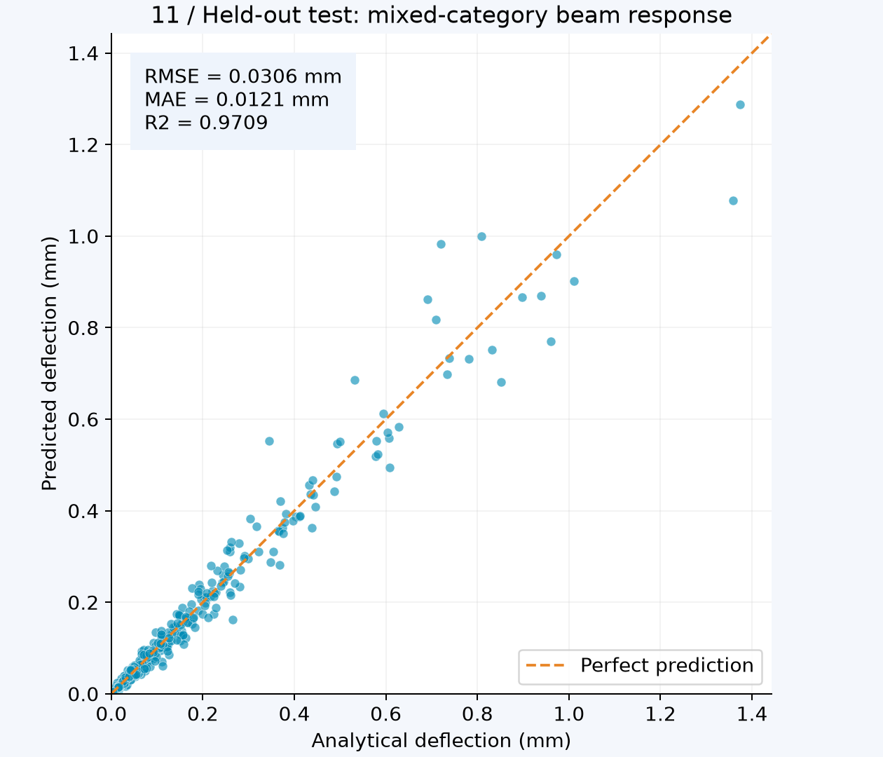

图11-3　混合类别梁响应预测

大多数样本接近理想预测线，但部分大挠度工况仍然出现明显偏差。

原因之一是大响应通常对应多个极端条件同时出现，例如：

• 较低弹性模量；
• 悬臂支承；
• 较大载荷；
• 较长梁；
• 较小截面高度。

这种参数组合在随机数据中相对较少。

---

十五、预测一个新的梁工况

输入：

\ F=3\\ \\mathrm{N} \\\ L=450\\ \\mathrm{mm} \\\ b=20\\ \\mathrm{mm}, \\qquad h=15\\ \\mathrm{mm} \\

材料为Steel，支承形式为Cantilever。

new_case = pd.DataFrame([{
    "F_N": 3.0,
    "L_mm": 450.0,
    "b_mm": 20.0,
    "h_mm": 15.0,
    "material": "Steel",
    "support": "Cantilever"
}])

predicted_u = model.predict(new_case)[0]

theoretical_u = (
    (1 / 3)
    * 3
    * 450**3
    / (
        210000
        * (20 * 15**3 / 12)
    )
)

print(f"理论挠度：{theoretical_u:.6f} mm")
print(f"预测挠度：{predicted_u:.6f} mm")

本次实际输出

理论挠度：0.077143 mm
预测挠度：0.074982 mm

该工况的绝对误差约为：

\ \|0.074982-0.077143\| = 0.002161\\ \\mathrm{mm} \\

---

十六、分析特征重要性

importance = model.get_feature_importance(
    train_pool
)

importance = importance / importance.sum()

order = np.argsort(importance)

plt.barh(
    np.array(feature_names)[order],
    importance[order]
)

plt.xlabel(
    "Normalized feature importance"
)

plt.tight_layout()
plt.show()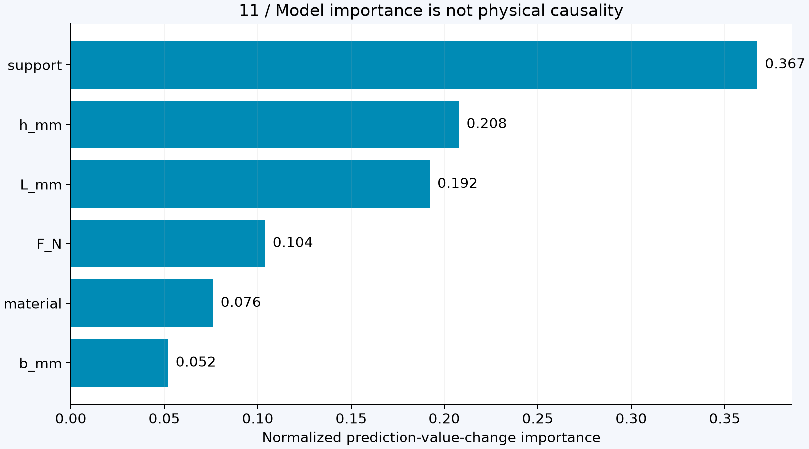

图11-4　CatBoost特征重要性

本次结果中，支承形式的重要性最高。这与两个理论公式之间的系数差异有关：

\ \\frac{1/3}{1/48}=16 \\

在相同材料、载荷和尺寸下，悬臂梁自由端挠度是对应简支梁跨中挠度的16倍。

但图中的重要性仍然是模型重要性，不是严格的物理贡献率：

\ \\text{特征重要性} \\neq \\text{物理因果贡献率} \\

---

十七、按支承类型分析残差

定义残差：

\ e_i=\\hat{u}_i-u_i \\

residual = (
    y_pred
    -
    y_test.to_numpy()
)

support_test = (
    X_test["support"].to_numpy()
)

for support, color in [
    ("Cantilever", "#008bb5"),
    ("SimplySupported", "#e88526")
]:
    mask = support_test == support

    plt.scatter(
        y_test.to_numpy()[mask],
        residual[mask],
        alpha=0.65,
        label=support,
        color=color
    )

plt.axhline(
    0,
    color="black",
    linestyle="--"
)

plt.xlabel("Analytical deflection (mm)")
plt.ylabel("Prediction - analytical (mm)")
plt.legend()
plt.grid(alpha=0.3)
plt.tight_layout()
plt.show()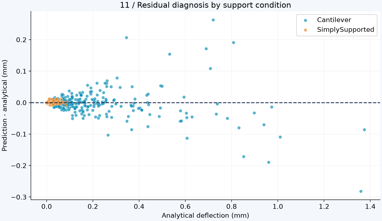

图11-5　不同支承条件的残差

图中可以看到：

• 简支梁挠度较小，残差集中在0附近；
• 悬臂梁覆盖更大的响应范围；
• 较大误差主要出现在悬臂梁高响应区域；
• 只看总体RMSE会掩盖类别之间的误差差异。

因此，对类别特征模型应进行分组评价：

\ \\operatorname{RMSE}_{\\mathrm{Steel}}, \\quad \\operatorname{RMSE}_{\\mathrm{Aluminum}}, \\quad \\operatorname{RMSE}_{\\mathrm{Titanium}} \\

以及：

\ \\operatorname{RMSE}_{\\mathrm{Cantilever}}, \\quad \\operatorname{RMSE}_{\\mathrm{SimplySupported}} \\

---

十八、遇到未见过的类别怎么办？

假设训练数据只有：

Steel
Aluminum
Titanium

预测时却输入：

Magnesium

程序可能仍然返回一个数值，但模型从未学习过镁合金对应的弹性模量和响应规律。

因此：

\ \\text{程序能够输出} \\neq \\text{模型具备可靠物理依据} \\

工程部署时应增加类别检查：

known_materials = {
    "Steel",
    "Aluminum",
    "Titanium"
}

material = "Magnesium"

if material not in known_materials:
    raise ValueError(
        f"未知材料类别：{material}"
    )

如果确实需要预测新材料，更合理的方法包括：

• 增加这种材料的训练数据；
• 把实际弹性模量作为数值输入；
• 使用材料成分或物理参数描述材料；
• 对新材料重新验证模型。

---

十九、真实有限元数据中的类别特征

CatBoost特别适合处理以下混合型CAE数据：

几何尺寸：
长度、厚度、孔径、裂纹长度

材料参数：
弹性模量、泊松比、屈服强度

类别信息：
材料名称、单元类型、接触类型、载荷类型

输出：
位移、应力、J积分、寿命

但类别变量必须具有明确含义。

例如，单元类型产生的响应差异可能反映：

• 单元理论不同；
• 积分方式不同；
• 网格密度不同；
• 剪切锁死或体积锁死；
• 数值误差尚未收敛。

不能简单把"模型识别出单元类型很重要"解释为真实结构的物理规律。

---

二十、常见误区

误区一：CatBoost只能用于分类

虽然名字中包含"Cat"，但它可以用于回归、分类和排序。本节使用的是：

CatBoostRegressor

误区二：类别越多越适合直接建模

如果一个类别只出现一两次，模型无法可靠学习其规律。应检查每个类别的样本数量。

误区三：类别名称包含物理知识

模型不会因为读到"Steel"这个单词就自动知道：

\ E=210000\\ \\text{MPa} \\

它只能从训练数据中学习统计关系。

误区四：设置早停一定会提前结束

本次实验设置了早停，但仍训练到3000轮上限附近。

误区五：可以用测试集选择参数

测试集只能进行最后评价。反复看测试结果再改参数，会导致测试集逐渐参与模型选择。

---

二十一、课后练习

基础练习

将材料改为两类：

materials = np.array([
    "Steel",
    "Aluminum"
])

重新训练，观察材料特征重要性是否变化。

进阶练习

增加一种支承形式，并给出相应解析公式或可信的有限元数据：

FixedFixed

检查新增类别在训练、验证和测试集中是否都有足够样本。

分组评价练习

分别计算三种材料的RMSE：

for material in materials:
    mask = (
        X_test["material"].to_numpy()
        == material
    )

    material_rmse = np.sqrt(
        mean_squared_error(
            y_test.to_numpy()[mask],
            y_pred[mask]
        )
    )

    print(
        material,
        material_rmse
    )

工程思考

如果已经拥有准确的弹性模量E，请比较两种输入方案：

方案一：

\ (F,L,b,h,\\text{material},\\text{support}) \\

方案二：

\ (F,L,E,b,h,\\text{support}) \\

思考哪一种方案更容易推广到训练数据中未出现过的新材料。

---

二十二、本节小结

本节完成了一个包含数值特征和类别特征的力学预测流程：

\ \\text{数值参数与类别条件} \\longrightarrow \\text{类别统计编码} \\longrightarrow \\text{Ordered Boosting} \\longrightarrow \\text{梁响应预测} \\longrightarrow \\text{分组误差诊断} \\

本节最重要的三点是：

1. 材料、支承和单元类型不能随意当作连续数字；
2. Ordered Boosting通过有序统计降低类别编码的目标泄漏风险；
3. 总体指标良好，不代表所有材料和边界条件都同样可靠。

最终应记住：

\ \\text{能够处理类别特征} \\neq \\text{自动理解类别的物理意义} \\

完整运行代码：

from pathlib import Path
from time import perf_counter
import json
import shutil
import numpy as np
import pandas as pd
import matplotlib
matplotlib.use("Agg")
import matplotlib.pyplot as plt
import catboost
from catboost import CatBoostRegressor, Pool
from sklearn.model_selection import train_test_split
from sklearn.metrics import mean_absolute_error, mean_squared_error, r2_score

OUT = Path(__file__).resolve().parent
FEATURES = ["F_N", "L_mm", "b_mm", "h_mm", "material", "support"]
CAT_FEATURES = ["material", "support"]

# Reproducible analytical teaching data. No artificial noise is added.
rng = np.random.default_rng(42)
n = 3000
materials = np.array(["Steel", "Aluminum", "Titanium"])
supports = np.array(["Cantilever", "SimplySupported"])
E_MAP = {"Steel": 210000.0, "Aluminum": 70000.0, "Titanium": 110000.0}
COEF_MAP = {"Cantilever": 1.0 / 3.0, "SimplySupported": 1.0 / 48.0}

df = pd.DataFrame({
    "F_N": rng.uniform(1, 5, n),
    "L_mm": rng.uniform(300, 600, n),
    "b_mm": rng.uniform(15, 30, n),
    "h_mm": rng.uniform(10, 20, n),
    "material": rng.choice(materials, n),
    "support": rng.choice(supports, n),
})
E = df["material"].map(E_MAP).to_numpy()
c = df["support"].map(COEF_MAP).to_numpy()
I = df["b_mm"].to_numpy() * df["h_mm"].to_numpy() ** 3 / 12.0
df["u_mm"] = c * df["F_N"].to_numpy() * df["L_mm"].to_numpy() ** 3 / (E * I)

# Stratify by the 3 x 2 category combinations, then split 60/20/20.
idx = np.arange(n)
strata = (df["material"] + "|" + df["support"]).to_numpy()
idx_dev, idx_test = train_test_split(
    idx, test_size=0.20, random_state=42, stratify=strata)
idx_train, idx_val = train_test_split(
    idx_dev, test_size=0.25, random_state=42, stratify=strata[idx_dev])
X_train, y_train = df.loc[idx_train, FEATURES], df.loc[idx_train, "u_mm"]
X_val, y_val = df.loc[idx_val, FEATURES], df.loc[idx_val, "u_mm"]
X_test, y_test = df.loc[idx_test, FEATURES], df.loc[idx_test, "u_mm"]

train_pool = Pool(X_train, y_train, cat_features=CAT_FEATURES)
val_pool = Pool(X_val, y_val, cat_features=CAT_FEATURES)
test_pool = Pool(X_test, y_test, cat_features=CAT_FEATURES)

model = CatBoostRegressor(
    loss_function="RMSE",
    eval_metric="RMSE",
    iterations=3000,
    learning_rate=0.03,
    depth=6,
    l2_leaf_reg=5.0,
    random_strength=0.5,
    boosting_type="Ordered",
    bootstrap_type="Bernoulli",
    subsample=0.85,
    random_seed=42,
    thread_count=2,
    allow_writing_files=False,
    verbose=False,
)

start = perf_counter()
model.fit(
    train_pool,
    eval_set=val_pool,
    early_stopping_rounds=100,
    use_best_model=True,
    verbose=False,
)
elapsed = perf_counter() - start

pred = model.predict(test_pool)
baseline = np.full(len(y_test), float(y_train.mean()))
rmse = float(np.sqrt(mean_squared_error(y_test, pred)))
mae = float(mean_absolute_error(y_test, pred))
r2 = float(r2_score(y_test, pred))
baseline_rmse = float(np.sqrt(mean_squared_error(y_test, baseline)))
residual = pred - y_test.to_numpy()
history = model.get_evals_result()

sample = pd.DataFrame([{
    "F_N": 3.0, "L_mm": 450.0, "b_mm": 20.0, "h_mm": 15.0,
    "material": "Steel", "support": "Cantilever",
}])
sample_true = (1 / 3) * 3 * 450**3 / (210000 * (20 * 15**3 / 12))
sample_pred = float(model.predict(sample)[0])

counts = df.loc[idx_test].groupby(["material", "support"], observed=True).size()
lines = [
    f"CatBoost version: {catboost.__version__}",
    f"Samples: train={len(y_train)}, validation={len(y_val)}, test={len(y_test)}",
    f"Test category combinations: {len(counts)} / 6; min count={int(counts.min())}",
    f"Best boosting round: {model.get_best_iteration() + 1}",
    f"Trees retained in model: {model.tree_count_}",
    f"Rounds evaluated before stopping: {len(history['learn']['RMSE'])}",
    f"Training wall time on this machine: {elapsed:.4f} s",
    f"Baseline RMSE: {baseline_rmse:.6f} mm",
    f"CatBoost RMSE: {rmse:.6f} mm",
    f"CatBoost MAE: {mae:.6f} mm",
    f"CatBoost R2: {r2:.6f}",
    f"Example theory: {sample_true:.6f} mm",
    f"Example prediction: {sample_pred:.6f} mm",
]
print("\n".join(lines))
(OUT / "run_results.txt").write_text("\n".join(lines), encoding="utf-8")
df.to_csv(OUT / "categorical_beam_dataset.csv", index=False, encoding="utf-8-sig")

# Save through an ASCII path first to avoid native-library Unicode path issues on Windows.
ascii_model = Path("work") / "lesson11_beam_catboost.cbm"
ascii_model.parent.mkdir(exist_ok=True)
model.save_model(str(ascii_model))
shutil.copy2(ascii_model, OUT / "beam_catboost.cbm")

plt.rcParams.update({
    "font.family": "DejaVu Sans", "font.size": 11,
    "axes.spines.top": False, "axes.spines.right": False,
    "figure.facecolor": "#f4f7fc", "axes.facecolor": "white",
})

# Figure 1: actual target distributions by material and support condition.
groups, labels = [], []
for material in materials:
    for support in supports:
        mask = (df["material"] == material) & (df["support"] == support)
        groups.append(df.loc[mask, "u_mm"].to_numpy())
        labels.append(f"{material[:2]}\n{support[:3]}")
fig, ax = plt.subplots(figsize=(10, 5.4), layout="constrained")
bp = ax.boxplot(groups, tick_labels=labels, patch_artist=True, showfliers=False)
for i, box in enumerate(bp["boxes"]):
    box.set_facecolor("#008bb5" if i % 2 == 0 else "#e88526")
    box.set_alpha(0.75)
ax.set(title="11 / Response distributions preserve category physics",
       xlabel="Material and support category", ylabel="Analytical maximum deflection (mm)")
ax.grid(axis="y", alpha=0.15)
fig.savefig(OUT / "01-category-response-distributions.png", dpi=180); plt.close(fig)

# Figure 2: actual learning curves.
rounds = np.arange(1, len(history["learn"]["RMSE"]) + 1)
fig, ax = plt.subplots(figsize=(10, 5.4), layout="constrained")
ax.plot(rounds, history["learn"]["RMSE"], color="#008bb5", label="Training")
ax.plot(rounds, history["validation"]["RMSE"], color="#e88526", label="Validation")
ax.axvline(model.get_best_iteration() + 1, color="#25365d", ls="--", lw=1.3,
           label=f"Best round: {model.get_best_iteration() + 1}")
ax.set(title="11 / CatBoost learning curves", xlabel="Boosting round", ylabel="RMSE (mm)")
ax.grid(alpha=0.15); ax.legend()
fig.savefig(OUT / "02-learning-curves.png", dpi=180); plt.close(fig)

# Figure 3: actual held-out predictions.
fig, ax = plt.subplots(figsize=(7, 6), layout="constrained")
ax.scatter(y_test, pred, s=27, alpha=0.62, color="#008bb5", edgecolors="white", linewidths=0.3)
limit = max(float(y_test.max()), float(pred.max())) * 1.05
ax.plot([0, limit], [0, limit], "--", color="#e88526", label="Perfect prediction")
ax.set(xlim=(0, limit), ylim=(0, limit), aspect="equal",
       title="11 / Held-out test: mixed-category beam response",
       xlabel="Analytical deflection (mm)", ylabel="Predicted deflection (mm)")
ax.text(0.05, 0.95, f"RMSE = {rmse:.4f} mm\nMAE = {mae:.4f} mm\nR2 = {r2:.4f}",
        transform=ax.transAxes, va="top",
        bbox={"facecolor": "#eef4fc", "edgecolor": "none", "pad": 8})
ax.grid(alpha=0.15); ax.legend(loc="lower right")
fig.savefig(OUT / "03-test-predictions.png", dpi=180); plt.close(fig)

# Figure 4: model feature importance (not causal importance).
scores = model.get_feature_importance(train_pool)
scores = scores / scores.sum()
order = np.argsort(scores)
fig, ax = plt.subplots(figsize=(9, 5), layout="constrained")
ax.barh(np.array(FEATURES)[order], scores[order], color="#008bb5")
for j, value in enumerate(scores[order]):
    ax.text(value + 0.004, j, f"{value:.3f}", va="center")
ax.set(xlabel="Normalized prediction-value-change importance",
       title="11 / Model importance is not physical causality")
ax.grid(axis="x", alpha=0.15)
fig.savefig(OUT / "04-feature-importance.png", dpi=180); plt.close(fig)

# Figure 5: actual residuals, colored by support category.
fig, ax = plt.subplots(figsize=(9, 5.2), layout="constrained")
support_test = X_test["support"].to_numpy()
for support, color in [("Cantilever", "#008bb5"), ("SimplySupported", "#e88526")]:
    mask = support_test == support
    ax.scatter(y_test.to_numpy()[mask], residual[mask], s=28, alpha=0.65,
               color=color, edgecolors="white", linewidths=0.3, label=support)
ax.axhline(0, color="#25365d", ls="--")
ax.set(title="11 / Residual diagnosis by support condition",
       xlabel="Analytical deflection (mm)", ylabel="Prediction - analytical (mm)")
ax.grid(alpha=0.15); ax.legend()
fig.savefig(OUT / "05-residuals-by-support.png", dpi=180); plt.close(fig)

metrics = {
    "catboost_version": catboost.__version__, "best_iteration": model.get_best_iteration() + 1,
    "trees_retained": model.tree_count_, "training_wall_time_seconds": elapsed,
    "baseline_rmse_mm": baseline_rmse, "test_rmse_mm": rmse,
    "test_mae_mm": mae, "test_r2": r2,
    "example_theory_mm": sample_true, "example_prediction_mm": sample_pred,
}
(OUT / "metrics.json").write_text(json.dumps(metrics, indent=2), encoding="utf-8")
print("Saved: dataset, model, metrics and five PNG figures.")

评价指标：

{

"catboost_version": "1.2.10",

"best_iteration": 2997,

"trees_retained": 2997,

"training_wall_time_seconds": 146.18879530020058,

"baseline_rmse_mm": 0.17977407002397702,

"test_rmse_mm": 0.030646784021649442,

"test_mae_mm": 0.012084176964269428,

"test_r2": 0.9709251145974431,

"example_theory_mm": 0.07714285714285714,

"example_prediction_mm": 0.07498205282714351

}

下一节将进入支持向量机与支持向量回归，研究昂贵高保真仿真条件下的小样本力学预测问题。