1.启动无人机程序的launch程序文件解释
1.<!-- 无人机初始位姿(出现的位置和朝向) -->
<arg name="x" default="0"/> <!-- 初始 x 坐标 -->
<arg name="y" default="0"/> <!-- 初始 y 坐标 -->
<arg name="z" default="0"/> <!-- 初始 z 坐标(高度) -->
<arg name="R" default="0"/> <!-- roll 翻滚角 -->
<arg name="P" default="0"/> <!-- pitch 俯仰角 -->
<arg name="Y" default="0"/> <!-- yaw 偏航角 -->
R:左右幅度摆动 P:前后幅度 Y绕z轴角度
<arg name="est" default="ekf2"/> <!-- 状态估计器(ekf2=扩展卡尔曼滤波,融合位置速度) -->
<arg name="vehicle" default="iris"/> <!-- 无人机型号(iris 是四旋翼) -->
<arg name="world" default="$(find mavlink_sitl_gazebo)/worlds/h11.world"/> <!-- 用哪个世界 -->
<arg name="sdf" default="$(find mavlink_sitl_gazebo)/models/iris_fpv_cam/iris_fpv_cam.sdf"/> <!-- 无人机的3D模型文件 --> 添加摄像头模型
模型大概意思 (这个简单懂就行,无非就是加入摄像头的时候需要用到)
2.无人机订阅相应数据,并在matlab中得到曲线
下面是进行操作
首先启动roslaunch px4 mavros_按住TAB键补全即可
然后在另外一个终端
bash
rosbag record -O flight_data.bag \
    /mavros/local_position/pose \
    /mavros/local_position/velocity_local
这个是官方自带的,rosbag相当于一个大容器,可以包含位置信息和速度信息,
打开第三个终端输入
bash
rosrun drone going飞行结束后,输入
bash
rosbag info flight_data.bag最后把 bag 转成 CSV,
单独提取位置话题转成 CSV
bash
rostopic echo -p /mavros/local_position/pose -b flight_data.bag > pose.csv.matlab程序如下:
Matlab
%% ============ 数据读取 ============
clear; clc; close all;

% 读取位置数据(跳过表头)
data = readmatrix('pose.csv', 'NumHeaderLines', 1);

% 列索引(重要!)
% 1=time(ns) 2=seq 3=stamp 4=frame_id(字符串) 5=x 6=y 7=z 8~11=四元数
t = (data(:,1) - data(1,1)) / 1e9;    % 时间 -> 秒
x = data(:,5);
y = data(:,6);
z = data(:,7);

%% ============ 绘图风格(顶刊常用)============
fontSize   = 11;                    % 字体大小
lineWidth  = 1.5;                   % 线宽
markerSize = 9;                     % 标记大小
cTrack = [0.00 0.45 0.74];          % 轨迹:蓝色
cStart = [0.47 0.67 0.19];          % 起点:绿色
cEnd   = [0.85 0.33 0.10];          % 终点:橙色

%% ============ 图1:3D 飞行轨迹 ============
figure('Color','w','Position',[80 80 620 520]);
plot3(x, y, z, '-', 'Color', cTrack, 'LineWidth', lineWidth);
hold on;
plot3(x(1), y(1), z(1), 'o', 'MarkerSize', markerSize, ...
    'MarkerFaceColor', cStart, 'MarkerEdgeColor','k', 'LineWidth',1);
plot3(x(end), y(end), z(end), 's', 'MarkerSize', markerSize, ...
    'MarkerFaceColor', cEnd, 'MarkerEdgeColor','k', 'LineWidth',1);
hold off;

xlabel('X (m)', 'FontSize', fontSize);
ylabel('Y (m)', 'FontSize', fontSize);
zlabel('Z (m)', 'FontSize', fontSize);
legend({'Trajectory','Start','End'}, 'Location','northeast', ...
    'FontSize', fontSize-1, 'Box','off');
grid on; box on; axis equal;
view(45, 22);                          % 3D 视角
set(gca, 'FontSize', fontSize, 'LineWidth', 0.8, 'TickDir','out');
% title('3D Flight Trajectory');        % 论文里一般不写标题

%% ============ 图2:俯视轨迹(XY 平面)============
figure('Color','w','Position',[720 80 500 460]);
plot(x, y, '-', 'Color', cTrack, 'LineWidth', lineWidth);
hold on;
plot(x(1), y(1), 'o', 'MarkerSize', markerSize, ...
    'MarkerFaceColor', cStart, 'MarkerEdgeColor','k');
plot(x(end), y(end), 's', 'MarkerSize', markerSize, ...
    'MarkerFaceColor', cEnd, 'MarkerEdgeColor','k');
hold off;

xlabel('X (m)', 'FontSize', fontSize);
ylabel('Y (m)', 'FontSize', fontSize);
legend({'Trajectory','Start','End'}, 'Location','best', ...
    'FontSize', fontSize-1, 'Box','off');
grid on; box on; axis equal;
set(gca, 'FontSize', fontSize, 'LineWidth', 0.8, 'TickDir','out');

%% ============ 图3:位置-时间曲线 ============
figure('Color','w','Position',[80 640 620 480]);
plot(t, x, '-', 'Color', [0.85 0.33 0.10], 'LineWidth', lineWidth); hold on;
plot(t, y, '-', 'Color', [0.47 0.67 0.19], 'LineWidth', lineWidth);
plot(t, z, '-', 'Color', [0.00 0.45 0.74], 'LineWidth', lineWidth);
hold off;

xlabel('Time (s)', 'FontSize', fontSize);
ylabel('Position (m)', 'FontSize', fontSize);
legend({'x','y','z'}, 'Location','northeast', ...
    'FontSize', fontSize-1, 'Box','off', 'NumColumns',3);
grid on; box on;
set(gca, 'FontSize', fontSize, 'LineWidth', 0.8, 'TickDir','out');
xlim([t(1) t(end)]);

%% ============ 导出为矢量图(投稿用)============
% 依次导出 3 个图(建议 PDF 矢量格式,插入 LaTeX 最清晰)
exportgraphics(gcf, 'trajectory_3d.pdf', 'ContentType','vector');
这个时候,你也在想那我输出速度的表格信息呢,该怎么操作,
也是一步不一样,导出这里
bash
# 导出位置(你之前做的)
rostopic echo -p /mavros/local_position/pose           -b flight_data.bag > pose.csv
#                ↑↑↑ 话题名(位置)

# 导出速度(把话题名换成 velocity_local)
rostopic echo -p /mavros/local_position/velocity_local -b flight_data.bag > vel.csv
#                ↑↑↑ 话题名(速度)
就是最后这里需要更改,matlab程序几乎相同,更改两点
Matlab
%% 原来读位置
data = readmatrix('pose.csv', 'NumHeaderLines', 1);
x = data(:,5);  y = data(:,6);  z = data(:,7);

%% 改成读速度(文件名换 + 变量名换,列号不变!)
vel = readmatrix('vel.csv', 'NumHeaderLines', 1);
vx = vel(:,5);  vy = vel(:,6);  vz = vel(:,7);
完整画速度曲线代码
Matlab
展示核心代码

%% ============ 顶刊大图(2x2)============
fig = figure('Color','w','Position',[60 60 900 700]);
tl = tiledlayout(2, 2, 'TileSpacing','compact', 'Padding','compact');

%% ---- (a) 三轴速度(原始+平滑叠加,评审最爱)----
nexttile;
% 原始数据:浅色细线(诚实展示)
plot(tv, vx, '-', 'Color', [cX 0.25], 'LineWidth', 0.8); hold on;
plot(tv, vy, '-', 'Color', [cY 0.25], 'LineWidth', 0.8);
plot(tv, vz, '-', 'Color', [cZ 0.25], 'LineWidth', 0.8);
% 平滑数据:深色粗线
plot(tv, vx_s, '-', 'Color', cX, 'LineWidth', lineWidth);
plot(tv, vy_s, '-', 'Color', cY, 'LineWidth', lineWidth);
plot(tv, vz_s, '-', 'Color', cZ, 'LineWidth', lineWidth);
hold off;

xlabel('Time (s)'); ylabel('Velocity (m/s)');
legend({'v_x','v_y','v_z'}, 'Location','best', 'FontSize', fontSize-2, ...
    'Box','off', 'NumColumns',3);
grid on; box on;
title('(a) Velocity Components', 'FontWeight','bold', 'FontSize', fontSize);
set(gca, 'LineWidth', 0.8, 'TickDir','out');

%% ---- (b) 总速度大小 |v| ----
nexttile;
% 原始(浅) + 平滑(深)
plot(tv, speed, '-', 'Color', [cS 0.20], 'LineWidth', 0.8); hold on;
plot(tv, speed_s, '-', 'Color', cS, 'LineWidth', lineWidth); hold off;

xlabel('Time (s)'); ylabel('Speed |v| (m/s)');
grid on; box on;
title('(b) Speed Magnitude', 'FontWeight','bold', 'FontSize', fontSize);
set(gca, 'LineWidth', 0.8, 'TickDir','out');

%% ---- (c) 速度-高度关系(相位图,更"高级")----
nexttile;
plot(vz_s, vx_s, '.', 'Color', cX, 'MarkerSize', 5);
xlabel('v_z (m/s)'); ylabel('v_x (m/s)');
grid on; box on; axis equal;
title('(c) Phase Portrait (v_x vs. v_z)', 'FontWeight','bold', 'FontSize', fontSize);
set(gca, 'LineWidth', 0.8, 'TickDir','out');

%% ---- (d) 速度分布直方图(展示统计特性)----
nexttile;
histogram(speed_s, 40, 'FaceColor', cS, 'EdgeColor','none', ...
    'FaceAlpha', 0.8);
xlabel('Speed |v| (m/s)'); ylabel('Count');
grid on; box on;
title('(d) Speed Distribution', 'FontWeight','bold', 'FontSize', fontSize);
set(gca, 'LineWidth', 0.8, 'TickDir','out');
四张图,高级图。这是对应解释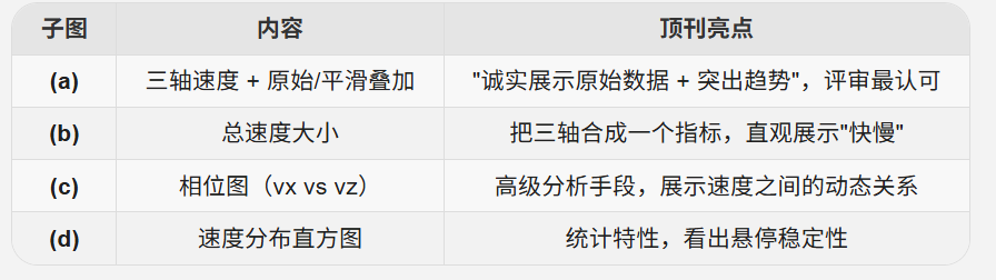
那么关于定点飞行一些科研绘图技巧和无人机模型解释,结束!