【深度学习】NLP，Transformer讲解，代码实战

文章目录

[1. 前言](#1. 前言)
[2. Transformer结构](#2. Transformer结构)
- - 训练过程
  - - [1. 输入嵌入和位置编码](#1. 输入嵌入和位置编码)
    - [2. 编码器层](#2. 编码器层)
    - - [2.1 单头的注意力机制(便于理解)](#2.1 单头的注意力机制(便于理解))
      - [2.2 多头的注意力机制(Transformer真实使用的)](#2.2 多头的注意力机制(Transformer真实使用的))
      - [2.3 残差连接和层归一化](#2.3 残差连接和层归一化)
      - [2.4 前馈神经网络（FFN）](#2.4 前馈神经网络（FFN）)
      - [2.5 残差连接和层归一化](#2.5 残差连接和层归一化)
      - [2.6 总结](#2.6 总结)
    - [3. 解码器层](#3. 解码器层)
  - 推理过程
  - - [1. 初始化](#1. 初始化)
    - [2. 编码器](#2. 编码器)
    - [3. 解码器逐步生成](#3. 解码器逐步生成)
    - [4. 输出生成](#4. 输出生成)
[3. 训练过程的代码](#3. 训练过程的代码)
[4. 推理过程的代码](#4. 推理过程的代码)
[5. 何为"多头"？](#5. 何为“多头”？)
[6. Mask如何给上去的？](#6. Mask如何给上去的？)
[7. 为何要位置编码？](#7. 为何要位置编码？)
[8. 为什么说Transformer可以并行化计算NLP任务？](#8. 为什么说Transformer可以并行化计算NLP任务？)
[9. MultiheadAttention的Pytorch官方代码](#9. MultiheadAttention的Pytorch官方代码)
[10. 何为QKV？](#10. 何为QKV？)
[11. 为何不是BN？](#11. 为何不是BN？)
[12. RNN的梯度消失是指什么？](#12. RNN的梯度消失是指什么？)
- - - RNN的梯度消失和其他模型的梯度消失有本质差别：
    - 如何降低RNN的梯度消失

1. 前言

来看一下Transformer结构。

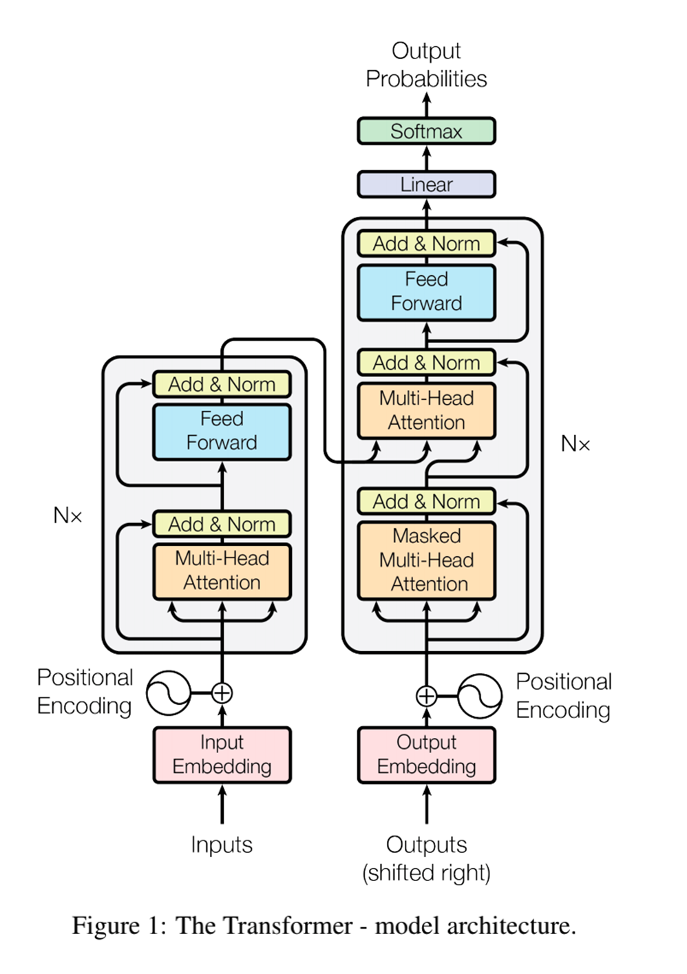
2. Transformer结构

表达Transformer模型从训练到推理的过程。

训练过程

1. 输入嵌入和位置编码

给定输入序列 X = [ x 1 , x 2 , ... , x n ] X = [x_1, x_2, \ldots, x_n] X=[x1,x2,...,xn] 和目标序列 Y = [ y 1 , y 2 , ... , y m ] Y = [y_1, y_2, \ldots, y_m] Y=[y1,y2,...,ym]，首先将它们转换为嵌入向量：
E x = [ E ( x 1 ) , E ( x 2 ) , ... , E ( x n ) ] E_x = [E(x_1), E(x_2), \ldots, E(x_n)] Ex=[E(x1),E(x2),...,E(xn)]
E y = [ E ( y 1 ) , E ( y 2 ) , ... , E ( y m ) ] E_y = [E(y_1), E(y_2), \ldots, E(y_m)] Ey=[E(y1),E(y2),...,E(ym)]

然后加上位置编码：

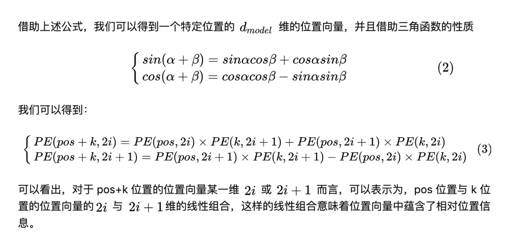
位置编码（Positional Encoding）用于表示序列中每个词的位置信息，帮助模型捕捉序列的顺序关系。Transformer使用了一种基于正弦和余弦函数的位置编码方式。

位置编码的具体公式如下：

对于输入序列中的第 i i i 个位置和第 j j j 个维度，位置编码为：

P ( i , 2 j ) = sin ⁡ ( i 1000 0 2 j / d model ) P(i, 2j) = \sin\left(\frac{i}{10000^{2j/d_{\text{model}}}}\right) P(i,2j)=sin(100002j/dmodeli)

P ( i , 2 j + 1 ) = cos ⁡ ( i 1000 0 2 j / d model ) P(i, 2j+1) = \cos\left(\frac{i}{10000^{2j/d_{\text{model}}}}\right) P(i,2j+1)=cos(100002j/dmodeli)

其中， d model d_{\text{model}} dmodel 是嵌入向量的维度。

将位置编码加到输入序列和目标序列的嵌入向量中：

P E x i = E ( x i ) + P ( i ) PE_{x_i} = E(x_i) + P(i) PExi=E(xi)+P(i)

P E y i = E ( y i ) + P ( i ) PE_{y_i} = E(y_i) + P(i) PEyi=E(yi)+P(i)

好好理解位置编码，第 i i i 个位置和第 j j j 个维度的数值是固定的编码，加到嵌入向量：

2. 编码器层

2.1 单头的注意力机制(便于理解)

编码器中的每一层包括一个多头自注意力机制和一个前馈神经网络：
Attention ( Q , K , V ) = softmax ( Q K T d k ) V \text{Attention}(Q, K, V) = \text{softmax}\left(\frac{QK^T}{\sqrt{d_k}}\right)V Attention(Q,K,V)=softmax(dk QKT)V

对于每个编码器层，我们有：
Self-Attention = Attention ( P E x , P E x , P E x ) \text{Self-Attention} = \text{Attention}(PE_x, PE_x, PE_x) Self-Attention=Attention(PEx,PEx,PEx)

在Transformer中，编码器和解码器都使用了自注意力机制（Self-Attention Mechanism）。在编码器中，查询（Query）、键（Key）和值（Value）矩阵都来自于输入的嵌入加上位置编码：

Q = K = V = P E x Q = K = V = PE_x Q=K=V=PEx

在解码器中，自注意力机制和编码器-解码器注意力机制都用到了类似的计算方式，区别在于解码器的自注意力机制是带掩码的，以防止每个时间步看到未来的信息。

2.2 多头的注意力机制(Transformer真实使用的)

在多头自注意力机制中，我们首先将嵌入向量投影到多个子空间，然后在每个子空间上计算注意力。每个头的注意力计算公式如下：

Attention ( Q , K , V ) = softmax ( Q K T d k ) V \text{Attention}(Q, K, V) = \text{softmax}\left(\frac{QK^T}{\sqrt{d_k}}\right)V Attention(Q,K,V)=softmax(dk QKT)V

对于多头注意力机制，我们有：
MultiHead ( Q , K , V ) = Concat ( head 1 , head 2 , ... , head h ) W O \text{MultiHead}(Q, K, V) = \text{Concat}(\text{head}_1, \text{head}_2, \ldots, \text{head}_h)W^O MultiHead(Q,K,V)=Concat(head1,head2,...,headh)WO

其中，
head i = Attention ( Q W i Q , K W i K , V W i V ) \text{head}_i = \text{Attention}(QW_i^Q, KW_i^K, VW_i^V) headi=Attention(QWiQ,KWiK,VWiV)

这里的 W i Q , W i K , W i V W_i^Q, W_i^K, W_i^V WiQ,WiK,WiV 是将输入投影到 i i i 头的参数矩阵， W O W^O WO 是输出的线性变换矩阵。

对于每个编码器层，我们有：
Self-Attention = MultiHead ( P E x , P E x , P E x ) \text{Self-Attention} = \text{MultiHead}(PE_x, PE_x, PE_x) Self-Attention=MultiHead(PEx,PEx,PEx)

Q = K = V = P E x Q = K = V = PE_x Q=K=V=PEx

所以，编码器层的自注意力机制具体为：
Self-Attention = MultiHead ( P E x , P E x , P E x ) \text{Self-Attention} = \text{MultiHead}(PE_x, PE_x, PE_x) Self-Attention=MultiHead(PEx,PEx,PEx)

2.3 残差连接和层归一化

残差连接和层归一化：
LayerOutput = LayerNorm ( x + MultiHead ( P E x , P E x , P E x ) ) \text{LayerOutput} = \text{LayerNorm}(x + \text{MultiHead}(PE_x, PE_x, PE_x)) LayerOutput=LayerNorm(x+MultiHead(PEx,PEx,PEx))

2.4 前馈神经网络（FFN）

前馈神经网络公式（FFN）：
FFN ( x ) = ReLU ( x W 1 + b 1 ) W 2 + b 2 \text{FFN}(x) = \text{ReLU}(xW_1 + b_1)W_2 + b_2 FFN(x)=ReLU(xW1+b1)W2+b2

2.5 残差连接和层归一化

LayerOutput = LayerNorm ( LayerOutput + FFN ( LayerOutput ) ) \text{LayerOutput} = \text{LayerNorm}(\text{LayerOutput} + \text{FFN}(\text{LayerOutput})) LayerOutput=LayerNorm(LayerOutput+FFN(LayerOutput))

2.6 总结

整个编码器层，在Transformer中可能是有多个的。

经过 L L L 层编码器，我们得到编码器的输出：
H = EncoderLayers ( P E x ) H = \text{EncoderLayers}(PE_x) H=EncoderLayers(PEx)

3. 解码器层

多头注意力机制：
MultiHead ( Q , K , V ) = Concat ( head 1 , head 2 , ... , head h ) W O \text{MultiHead}(Q, K, V) = \text{Concat}(\text{head}_1, \text{head}_2, \ldots, \text{head}_h)W^O MultiHead(Q,K,V)=Concat(head1,head2,...,headh)WO

其中每个头的计算为：
head i = Attention ( Q W i Q , K W i K , V W i V ) \text{head}_i = \text{Attention}(QW_i^Q, KW_i^K, VW_i^V) headi=Attention(QWiQ,KWiK,VWiV)

带掩码的自注意力机制：
Masked-Attention ( Q , K , V ) = softmax ( Q K T + M d k ) V \text{Masked-Attention}(Q, K, V) = \text{softmax}\left(\frac{QK^T + M}{\sqrt{d_k}}\right)V Masked-Attention(Q,K,V)=softmax(dk QKT+M)V

其中 M M M 是掩码矩阵，掩盖未来时间步。

注意了，与编码器的交互里，在这里Q是解码器的输出，编码器的输出作为K和V。

Attention ( Q , K , V ) = softmax ( Q K T d k ) V \text{Attention}(Q, K, V) = \text{softmax}\left(\frac{QK^T}{\sqrt{d_k}}\right)V Attention(Q,K,V)=softmax(dk QKT)V

前馈神经网络：
FFN ( x ) = ReLU ( x W 1 + b 1 ) W 2 + b 2 \text{FFN}(x) = \text{ReLU}(xW_1 + b_1)W_2 + b_2 FFN(x)=ReLU(xW1+b1)W2+b2

残差连接和层归一化：
LayerOutput = LayerNorm ( x + FFN ( MultiHead ( P E y , P E y , P E y ) + P E y ) ) \text{LayerOutput} = \text{LayerNorm}(x + \text{FFN}(\text{MultiHead}(PE_y, PE_y, PE_y) + PE_y)) LayerOutput=LayerNorm(x+FFN(MultiHead(PEy,PEy,PEy)+PEy))

经过 L L L 层解码器，我们得到解码器的输出：
D = DecoderLayers ( P E y ) D = \text{DecoderLayers}(PE_y) D=DecoderLayers(PEy)

通过线性变换和Softmax层生成最终的词概率分布：
Logits = D ⋅ W o + b o \text{Logits} = D \cdot W_o + b_o Logits=D⋅Wo+bo
OutputProbabilities = softmax ( Logits ) \text{OutputProbabilities} = \text{softmax}(\text{Logits}) OutputProbabilities=softmax(Logits)

推理过程

1. 初始化

初始化输入序列 X = [ x 1 , x 2 , ... , x n ] X = [x_1, x_2, \ldots, x_n] X=[x1,x2,...,xn]，目标序列开始标记为 Y = [ sos ] Y = [\text{sos}] Y=[sos]。

2. 编码器

编码器部分同训练过程：
H = EncoderLayers ( P E x ) H = \text{EncoderLayers}(PE_x) H=EncoderLayers(PEx)

3. 解码器逐步生成

带掩码的多头自注意力机制：
Masked-MultiHead-Attention ( Q , K , V ) = MultiHead ( Q , K , V ) \text{Masked-MultiHead-Attention}(Q, K, V) = \text{MultiHead}(Q, K, V) Masked-MultiHead-Attention(Q,K,V)=MultiHead(Q,K,V)

编码器-解码器多头注意力机制：
Enc-Dec-MultiHead-Attention ( Q , K , V ) = MultiHead ( Q , K , V ) \text{Enc-Dec-MultiHead-Attention}(Q, K, V) = \text{MultiHead}(Q, K, V) Enc-Dec-MultiHead-Attention(Q,K,V)=MultiHead(Q,K,V)

残差连接和层归一化：
LayerOutput = LayerNorm ( x + Masked-MultiHead-Attention ( P E y ) + P E y ) \text{LayerOutput} = \text{LayerNorm}(x + \text{Masked-MultiHead-Attention}(PE_y) + PE_y) LayerOutput=LayerNorm(x+Masked-MultiHead-Attention(PEy)+PEy)

然后，经过前馈神经网络：
LayerOutput = LayerNorm ( LayerOutput + FFN ( LayerOutput + Enc-Dec-MultiHead-Attention ( P E y , H , H ) ) ) \text{LayerOutput} = \text{LayerNorm}(\text{LayerOutput} + \text{FFN}(\text{LayerOutput} + \text{Enc-Dec-MultiHead-Attention}(PE_y, H, H))) LayerOutput=LayerNorm(LayerOutput+FFN(LayerOutput+Enc-Dec-MultiHead-Attention(PEy,H,H)))

经过 L L L 层解码器，我们得到解码器的输出：
D = DecoderLayers ( P E y , H ) D = \text{DecoderLayers}(PE_y, H) D=DecoderLayers(PEy,H)

4. 输出生成

通过线性变换和Softmax层生成最终的词概率分布：
Logits = D ⋅ W o + b o \text{Logits} = D \cdot W_o + b_o Logits=D⋅Wo+bo

OutputProbabilities = softmax ( Logits ) \text{OutputProbabilities} = \text{softmax}(\text{Logits}) OutputProbabilities=softmax(Logits)

3. 训练过程的代码

不算batch的概念进去：

cpp 复制代码

import numpy as np

# 设置随机种子以确保可重复性
np.random.seed(42)

# 模拟输入序列和目标序列
input_seq_len = 5
target_seq_len = 5
d_model = 4  # 嵌入维度

input_seq = np.random.randint(0, 10, (input_seq_len,))
target_seq = np.random.randint(0, 10, (target_seq_len,))

# 模拟嵌入矩阵
embedding_matrix = np.random.rand(10, d_model)  # 词汇表大小为10

# 输入嵌入
input_embeddings = embedding_matrix[input_seq]
target_embeddings = embedding_matrix[target_seq]

# 位置编码
def get_positional_encoding(seq_len, d_model):
    pos_enc = np.zeros((seq_len, d_model))
    for pos in range(seq_len):
        for i in range(d_model):
            if i % 2 == 0:
                pos_enc[pos, i] = np.sin(pos / (10000 ** (2 * i / d_model)))
            else:
                pos_enc[pos, i] = np.cos(pos / (10000 ** (2 * (i - 1) / d_model)))
    return pos_enc

input_pos_enc = get_positional_encoding(input_seq_len, d_model)
target_pos_enc = get_positional_encoding(target_seq_len, d_model)

# 添加位置编码到嵌入
input_embeddings += input_pos_enc
target_embeddings += target_pos_enc

# 编码器层：自注意力机制和前馈神经网络
def self_attention(Q, K, V):
    d_k = Q.shape[-1]
    scores = np.dot(Q, K.T) / np.sqrt(d_k)
    attention_weights = np.exp(scores) / np.sum(np.exp(scores), axis=-1, keepdims=True)
    return np.dot(attention_weights, V)

def feed_forward(x):
    W1 = np.random.rand(d_model, d_model)
    b1 = np.random.rand(d_model)
    W2 = np.random.rand(d_model, d_model)
    b2 = np.random.rand(d_model)
    return np.dot(np.maximum(0, np.dot(x, W1) + b1), W2) + b2

# 单个编码器层
def encoder_layer(x):
    attn_output = self_attention(x, x, x)
    attn_output += x  # 残差连接
    norm_output = attn_output / np.linalg.norm(attn_output, axis=-1, keepdims=True)
    ff_output = feed_forward(norm_output)
    ff_output += norm_output  # 残差连接
    return ff_output / np.linalg.norm(ff_output, axis=-1, keepdims=True)

# 编码器
encoder_output = input_embeddings
for _ in range(2):  # 使用2层编码器
    encoder_output = encoder_layer(encoder_output)

# 解码器层：带掩码的自注意力机制、编码器-解码器注意力机制和前馈神经网络
def masked_self_attention(Q, K, V):
    mask = np.triu(np.ones((Q.shape[0], K.shape[0])), k=1)  # 上三角掩码
    d_k = Q.shape[-1]
    scores = np.dot(Q, K.T) / np.sqrt(d_k)
    scores -= mask * 1e9  # 应用掩码
    attention_weights = np.exp(scores) / np.sum(np.exp(scores), axis=-1, keepdims=True)
    return np.dot(attention_weights, V)

# 单个解码器层
def decoder_layer(x, enc_output):
    masked_attn_output = masked_self_attention(x, x, x)
    masked_attn_output += x  # 残差连接
    norm_output1 = masked_attn_output / np.linalg.norm(masked_attn_output, axis=-1, keepdims=True)
    
    enc_dec_attn_output = self_attention(norm_output1, enc_output, enc_output)
    enc_dec_attn_output += norm_output1  # 残差连接
    norm_output2 = enc_dec_attn_output / np.linalg.norm(enc_dec_attn_output, axis=-1, keepdims=True)
    
    ff_output = feed_forward(norm_output2)
    ff_output += norm_output2  # 残差连接
    return ff_output / np.linalg.norm(ff_output, axis=-1, keepdims=True)

# 解码器
decoder_output = target_embeddings
for _ in range(2):  # 使用2层解码器
    decoder_output = decoder_layer(decoder_output, encoder_output)

# 线性变换和Softmax层
output_vocab_size = 10
linear_transform = np.random.rand(d_model, output_vocab_size)
logits = np.dot(decoder_output, linear_transform)
output_probs = np.exp(logits) / np.sum(np.exp(logits), axis=-1, keepdims=True)

# 输出结果
print("Input Sequence:", input_seq)
print("Target Sequence (shifted):", target_seq)
print("Output Probabilities:\n", output_probs)

多头注意力机制：

cpp 复制代码

import numpy as np

# 设置随机种子以确保可重复性
np.random.seed(42)

# 模拟输入序列和目标序列
input_seq_len = 5
target_seq_len = 5
d_model = 4  # 嵌入维度
num_heads = 2  # 注意力头的数量

input_seq = np.random.randint(0, 10, (input_seq_len,))
target_seq = np.random.randint(0, 10, (target_seq_len,))

# 模拟嵌入矩阵
embedding_matrix = np.random.rand(10, d_model)  # 词汇表大小为10

# 输入嵌入
input_embeddings = embedding_matrix[input_seq]
target_embeddings = embedding_matrix[target_seq]


# 位置编码
def get_positional_encoding(seq_len, d_model):
    pos_enc = np.zeros((seq_len, d_model))
    for pos in range(seq_len):
        for i in range(d_model):
            if i % 2 == 0:
                pos_enc[pos, i] = np.sin(pos / (10000 ** (2 * i / d_model)))
            else:
                pos_enc[pos, i] = np.cos(pos / (10000 ** (2 * (i - 1) / d_model)))
    return pos_enc


input_pos_enc = get_positional_encoding(input_seq_len, d_model)
target_pos_enc = get_positional_encoding(target_seq_len, d_model)

# 添加位置编码到嵌入
input_embeddings += input_pos_enc
target_embeddings += target_pos_enc


# 多头注意力机制
def multi_head_attention(Q, K, V, num_heads):
    d_k = Q.shape[-1] // num_heads
    all_heads = []
    for i in range(num_heads):
        # 分头处理
        Q_head = Q[:, i * d_k:(i + 1) * d_k]
        K_head = K[:, i * d_k:(i + 1) * d_k]
        V_head = V[:, i * d_k:(i + 1) * d_k]
        # 计算单头注意力
        scores = np.dot(Q_head, K_head.T) / np.sqrt(d_k)
        attention_weights = np.exp(scores) / np.sum(np.exp(scores), axis=-1, keepdims=True)
        head_output = np.dot(attention_weights, V_head)
        all_heads.append(head_output)
    # 拼接所有头的输出
    multi_head_output = np.concatenate(all_heads, axis=-1)
    return multi_head_output


def feed_forward(x):
    W1 = np.random.rand(d_model, d_model)
    b1 = np.random.rand(d_model)
    W2 = np.random.rand(d_model, d_model)
    b2 = np.random.rand(d_model)
    return np.dot(np.maximum(0, np.dot(x, W1) + b1), W2) + b2


# 单个编码器层
def encoder_layer(x, num_heads):
    attn_output = multi_head_attention(x, x, x, num_heads)
    attn_output += x  # 残差连接
    norm_output = attn_output / np.linalg.norm(attn_output, axis=-1, keepdims=True)
    ff_output = feed_forward(norm_output)
    ff_output += norm_output  # 残差连接
    return ff_output / np.linalg.norm(ff_output, axis=-1, keepdims=True)


# 编码器
encoder_output = input_embeddings
for _ in range(2):  # 使用2层编码器
    encoder_output = encoder_layer(encoder_output, num_heads)


# 带掩码的多头注意力机制
def masked_multi_head_attention(Q, K, V, num_heads):
    mask = np.triu(np.ones((Q.shape[0], K.shape[0])), k=1)  # 上三角掩码
    d_k = Q.shape[-1] // num_heads
    all_heads = []
    for i in range(num_heads):
        # 分头处理
        Q_head = Q[:, i * d_k:(i + 1) * d_k]
        K_head = K[:, i * d_k:(i + 1) * d_k]
        V_head = V[:, i * d_k:(i + 1) * d_k]
        # 计算单头带掩码注意力
        scores = np.dot(Q_head, K_head.T) / np.sqrt(d_k)
        scores -= mask * 1e9  # 应用掩码
        attention_weights = np.exp(scores) / np.sum(np.exp(scores), axis=-1, keepdims=True)
        head_output = np.dot(attention_weights, V_head)
        all_heads.append(head_output)
    # 拼接所有头的输出
    multi_head_output = np.concatenate(all_heads, axis=-1)
    return multi_head_output


# 单个解码器层
def decoder_layer(x, enc_output, num_heads):
    masked_attn_output = masked_multi_head_attention(x, x, x, num_heads)
    masked_attn_output += x  # 残差连接
    norm_output1 = masked_attn_output / np.linalg.norm(masked_attn_output, axis=-1, keepdims=True)

    enc_dec_attn_output = multi_head_attention(norm_output1, enc_output, enc_output, num_heads)
    enc_dec_attn_output += norm_output1  # 残差连接
    norm_output2 = enc_dec_attn_output / np.linalg.norm(enc_dec_attn_output, axis=-1, keepdims=True)

    ff_output = feed_forward(norm_output2)
    ff_output += norm_output2  # 残差连接
    return ff_output / np.linalg.norm(ff_output, axis=-1, keepdims=True)


# 解码器
decoder_output = target_embeddings
for _ in range(2):  # 使用2层解码器
    decoder_output = decoder_layer(decoder_output, encoder_output, num_heads)

# 线性变换和Softmax层
output_vocab_size = 10
linear_transform = np.random.rand(d_model, output_vocab_size)
logits = np.dot(decoder_output, linear_transform)
output_probs = np.exp(logits) / np.sum(np.exp(logits), axis=-1, keepdims=True)

# 输出结果
print("Input Sequence:", input_seq)
print("Target Sequence (shifted):", target_seq)
print("Output Probabilities:\n", output_probs)

4. 推理过程的代码

不算batch的概念进去：

cpp 复制代码

import numpy as np

# 设置随机种子以确保可重复性
np.random.seed(42)

# 模拟输入序列
input_seq_len = 5
d_model = 4  # 嵌入维度
vocab_size = 10
max_seq_len = 10  # 生成序列的最大长度

input_seq = np.random.randint(0, vocab_size, (input_seq_len,))

# 模拟嵌入矩阵
embedding_matrix = np.random.rand(vocab_size, d_model)

# 输入嵌入
input_embeddings = embedding_matrix[input_seq]

# 位置编码
def get_positional_encoding(seq_len, d_model):
    pos_enc = np.zeros((seq_len, d_model))
    for pos in range(seq_len):
        for i in range(d_model):
            if i % 2 == 0:
                pos_enc[pos, i] = np.sin(pos / (10000 ** (2 * i / d_model)))
            else:
                pos_enc[pos, i] = np.cos(pos / (10000 ** (2 * (i - 1) / d_model)))
    return pos_enc

input_pos_enc = get_positional_encoding(input_seq_len, d_model)
input_embeddings += input_pos_enc

# 编码器层：自注意力机制和前馈神经网络
def self_attention(Q, K, V):
    d_k = Q.shape[-1]
    scores = np.dot(Q, K.T) / np.sqrt(d_k)
    attention_weights = np.exp(scores) / np.sum(np.exp(scores), axis=-1, keepdims=True)
    return np.dot(attention_weights, V)

def feed_forward(x):
    W1 = np.random.rand(d_model, d_model)
    b1 = np.random.rand(d_model)
    W2 = np.random.rand(d_model, d_model)
    b2 = np.random.rand(d_model)
    return np.dot(np.maximum(0, np.dot(x, W1) + b1), W2) + b2

# 单个编码器层
def encoder_layer(x):
    attn_output = self_attention(x, x, x)
    attn_output += x  # 残差连接
    norm_output = attn_output / np.linalg.norm(attn_output, axis=-1, keepdims=True)
    ff_output = feed_forward(norm_output)
    ff_output += norm_output  # 残差连接
    return ff_output / np.linalg.norm(ff_output, axis=-1, keepdims=True)

# 编码器
encoder_output = input_embeddings
for _ in range(2):  # 使用2层编码器
    encoder_output = encoder_layer(encoder_output)

# 解码器层：带掩码的自注意力机制、编码器-解码器注意力机制和前馈神经网络
def masked_self_attention(Q, K, V):
    mask = np.triu(np.ones((Q.shape[0], K.shape[0])), k=1)  # 上三角掩码
    d_k = Q.shape[-1]
    scores = np.dot(Q, K.T) / np.sqrt(d_k)
    scores -= mask * 1e9  # 应用掩码
    attention_weights = np.exp(scores) / np.sum(np.exp(scores), axis=-1, keepdims=True)
    return np.dot(attention_weights, V)

# 单个解码器层
def decoder_layer(x, enc_output):
    masked_attn_output = masked_self_attention(x, x, x)
    masked_attn_output += x  # 残差连接
    norm_output1 = masked_attn_output / np.linalg.norm(masked_attn_output, axis=-1, keepdims=True)
    
    enc_dec_attn_output = self_attention(norm_output1, enc_output, enc_output)
    enc_dec_attn_output += norm_output1  # 残差连接
    norm_output2 = enc_dec_attn_output / np.linalg.norm(enc_dec_attn_output, axis=-1, keepdims=True)
    
    ff_output = feed_forward(norm_output2)
    ff_output += norm_output2  # 残差连接
    return ff_output / np.linalg.norm(ff_output, axis=-1, keepdims=True)

# 生成序列
def generate_sequence(encoder_output, start_token, vocab_size, max_seq_len):
    generated_seq = [start_token]
    for _ in range(max_seq_len - 1):
        target_embeddings = embedding_matrix[generated_seq]
        target_pos_enc = get_positional_encoding(len(generated_seq), d_model)
        target_embeddings += target_pos_enc
        
        decoder_output = target_embeddings
        for _ in range(2):  # 使用2层解码器
            decoder_output = decoder_layer(decoder_output, encoder_output)
        
        logits = np.dot(decoder_output[-1], np.random.rand(d_model, vocab_size))  # 只看最后一个时间步
        next_token = np.argmax(logits)  # 选取概率最高的词
        generated_seq.append(next_token)
        
        if next_token == 2:  # 假设2是<eos>结束标记
            break
    
    return generated_seq

# 生成翻译序列
start_token = 1  # 假设1是<sos>开始标记
translated_sequence = generate_sequence(encoder_output, start_token, vocab_size, max_seq_len)
print("Translated Sequence:", translated_sequence)

加入多头注意力：

cpp 复制代码

import numpy as np

# 设置随机种子以确保可重复性
np.random.seed(42)

# 模拟输入序列
input_seq_len = 5
d_model = 4  # 嵌入维度
num_heads = 2  # 注意力头的数量
vocab_size = 10
max_seq_len = 10  # 生成序列的最大长度

input_seq = np.random.randint(0, vocab_size, (input_seq_len,))

# 模拟嵌入矩阵
embedding_matrix = np.random.rand(vocab_size, d_model)

# 输入嵌入
input_embeddings = embedding_matrix[input_seq]

# 位置编码
def get_positional_encoding(seq_len, d_model):
    pos_enc = np.zeros((seq_len, d_model))
    for pos in range(seq_len):
        for i in range(d_model):
            if i % 2 == 0:
                pos_enc[pos, i] = np.sin(pos / (10000 ** (2 * i / d_model)))
            else:
                pos_enc[pos, i] = np.cos(pos / (10000 ** (2 * (i - 1) / d_model)))
    return pos_enc

input_pos_enc = get_positional_encoding(input_seq_len, d_model)
input_embeddings += input_pos_enc

# 多头注意力机制
def multi_head_attention(Q, K, V, num_heads):
    d_k = Q.shape[-1] // num_heads
    all_heads = []
    for i in range(num_heads):
        # 分头处理
        Q_head = Q[:, i * d_k:(i + 1) * d_k]
        K_head = K[:, i * d_k:(i + 1) * d_k]
        V_head = V[:, i * d_k:(i + 1) * d_k]
        # 计算单头注意力
        scores = np.dot(Q_head, K_head.T) / np.sqrt(d_k)
        attention_weights = np.exp(scores) / np.sum(np.exp(scores), axis=-1, keepdims=True)
        head_output = np.dot(attention_weights, V_head)
        all_heads.append(head_output)
    # 拼接所有头的输出
    multi_head_output = np.concatenate(all_heads, axis=-1)
    return multi_head_output

def feed_forward(x):
    W1 = np.random.rand(d_model, d_model)
    b1 = np.random.rand(d_model)
    W2 = np.random.rand(d_model, d_model)
    b2 = np.random.rand(d_model)
    return np.dot(np.maximum(0, np.dot(x, W1) + b1), W2) + b2

# 单个编码器层
def encoder_layer(x, num_heads):
    attn_output = multi_head_attention(x, x, x, num_heads)
    attn_output += x  # 残差连接
    norm_output = attn_output / np.linalg.norm(attn_output, axis=-1, keepdims=True)
    ff_output = feed_forward(norm_output)
    ff_output += norm_output  # 残差连接
    return ff_output / np.linalg.norm(ff_output, axis=-1, keepdims=True)

# 编码器
encoder_output = input_embeddings
for _ in range(2):  # 使用2层编码器
    encoder_output = encoder_layer(encoder_output, num_heads)

# 带掩码的多头注意力机制
def masked_multi_head_attention(Q, K, V, num_heads):
    mask = np.triu(np.ones((Q.shape[0], K.shape[0])), k=1)  # 上三角掩码
    d_k = Q.shape[-1] // num_heads
    all_heads = []
    for i in range(num_heads):
        # 分头处理
        Q_head = Q[:, i * d_k:(i + 1) * d_k]
        K_head = K[:, i * d_k:(i + 1) * d_k]
        V_head = V[:, i * d_k:(i + 1) * d_k]
        # 计算单头带掩码注意力
        scores = np.dot(Q_head, K_head.T) / np.sqrt(d_k)
        scores -= mask * 1e9  # 应用掩码
        attention_weights = np.exp(scores) / np.sum(np.exp(scores), axis=-1, keepdims=True)
        head_output = np.dot(attention_weights, V_head)
        all_heads.append(head_output)
    # 拼接所有头的输出
    multi_head_output = np.concatenate(all_heads, axis=-1)
    return multi_head_output

# 单个解码器层
def decoder_layer(x, enc_output, num_heads):
    masked_attn_output = masked_multi_head_attention(x, x, x, num_heads)
    masked_attn_output += x  # 残差连接
    norm_output1 = masked_attn_output / np.linalg.norm(masked_attn_output, axis=-1, keepdims=True)
    
    enc_dec_attn_output = multi_head_attention(norm_output1, enc_output, enc_output, num_heads)
    enc_dec_attn_output += norm_output1  # 残差连接
    norm_output2 = enc_dec_attn_output / np.linalg.norm(enc_dec_attn_output, axis=-1, keepdims=True)
    
    ff_output = feed_forward(norm_output2)
    ff_output += norm_output2  # 残差连接
    return ff_output / np.linalg.norm(ff_output, axis=-1, keepdims=True)

# 生成序列
def generate_sequence(encoder_output, start_token, vocab_size, max_seq_len, num_heads):
    generated_seq = [start_token]
    for _ in range(max_seq_len - 1):
        target_embeddings = embedding_matrix[generated_seq]
        target_pos_enc = get_positional_encoding(len(generated_seq), d_model)
        target_embeddings += target_pos_enc
        
        decoder_output = target_embeddings
        for _ in range(2):  # 使用2层解码器
            decoder_output = decoder_layer(decoder_output, encoder_output, num_heads)
        
        logits = np.dot(decoder_output[-1], np.random.rand(d_model, vocab_size))  # 只看最后一个时间步
        next_token = np.argmax(logits)  # 选取概率最高的词
        generated_seq.append(next_token)
        
        if next_token == 2:  # 假设2是<eos>结束标记
            break
    
    return generated_seq

# 生成翻译序列
start_token = 1  # 假设1是<sos>开始标记
translated_sequence = generate_sequence(encoder_output, start_token, vocab_size, max_seq_len, num_heads)
print("Translated Sequence:", translated_sequence)

5. 何为"多头"？

多头注意力机制允许模型在不同的表示子空间中同时关注不同的位置。

通过将输入的查询、键和值矩阵拆分为多个头，模型能够并行地学习多组注意力权重，每组都专注于不同的表示子空间。这有助于模型更好地捕获输入序列中的复杂关系。

举个例子来说，Transformer编码器模型里面设置特征维度如果是768，头是12头，那么每个头去管理768/12=64个特征，

让我们结合公式和代码来理解多头注意力机制是如何工作的：

首先，我们定义了多头注意力机制的函数，其输入包括查询矩阵 ( Q )，键矩阵 ( K )，值矩阵 ( V )，以及头的数量（num_heads）。
在函数内部，我们计算每个头的维度 ( d_k )，这是根据查询矩阵的最后一个维度除以头的数量得到的。
接下来，我们循环遍历每个头。在每个头中，我们将查询、键和值矩阵分别切片成 ( num_heads ) 个部分，然后分别用于计算单独的注意力权重。
注意力权重的计算公式是根据公式中的：
scores = Q K T d k \text{scores} = \frac{QK^T}{\sqrt{d_k}} scores=dk QKT

进行计算的。在代码中，我们计算每个头的分数矩阵，并应用了缩放因子 ( \sqrt{d_k} )。然后，我们使用 softmax 函数将分数转换为注意力权重。
每个头的注意力权重被用来加权值矩阵，然后进行加权求和，得到头的输出。
最后，我们将所有头的输出连接起来，形成多头注意力机制的最终输出。连接是在最后一个维度上进行的，确保了每个头的输出都被保持在同一位置。

在多头注意力机制中，将所有头的输出连接起来时，通常是在最后一个维度上进行连接，也就是说特征是横着连接的。假设每个头的输出维度为 d k d_k dk，头的数量为 n u m _ h e a d s num\_heads num_heads，那么每个头的输出将是一个形状为 ( batch_size , seq_length , d k ) (\text{batch\_size}, \text{seq\_length}, d_k) (batch_size,seq_length,dk) 的张量。连接所有头的输出时，我们将它们在最后一个维度上拼接起来，形成一个形状为 ( batch_size , seq_length , d k × n u m _ h e a d s ) (\text{batch\_size}, \text{seq\_length}, d_k \times num\_heads) (batch_size,seq_length,dk×num_heads) 的张量。

代码：

cpp 复制代码

# 多头注意力机制
def multi_head_attention(Q, K, V, num_heads):
    d_k = Q.shape[-1] // num_heads
    all_heads = []
    for i in range(num_heads):
        # 分头处理
        Q_head = Q[:, i * d_k:(i + 1) * d_k]
        K_head = K[:, i * d_k:(i + 1) * d_k]
        V_head = V[:, i * d_k:(i + 1) * d_k]
        # 计算单头注意力
        scores = np.dot(Q_head, K_head.T) / np.sqrt(d_k)
        attention_weights = np.exp(scores) / np.sum(np.exp(scores), axis=-1, keepdims=True)
        head_output = np.dot(attention_weights, V_head)
        all_heads.append(head_output)
    # 拼接所有头的输出
    multi_head_output = np.concatenate(all_heads, axis=-1)
    return multi_head_output

6. Mask如何给上去的？

mask是上三角掩码，给入的时候是scores -= mask * 1e9 # 应用掩码，代码如下：

cpp 复制代码

# 带掩码的多头注意力机制
def masked_multi_head_attention(Q, K, V, num_heads):
    mask = np.triu(np.ones((Q.shape[0], K.shape[0])), k=1)  # 上三角掩码
    d_k = Q.shape[-1] // num_heads
    all_heads = []
    for i in range(num_heads):
        # 分头处理
        Q_head = Q[:, i * d_k:(i + 1) * d_k]
        K_head = K[:, i * d_k:(i + 1) * d_k]
        V_head = V[:, i * d_k:(i + 1) * d_k]
        # 计算单头带掩码注意力
        scores = np.dot(Q_head, K_head.T) / np.sqrt(d_k)
        scores -= mask * 1e9  # 应用掩码
        attention_weights = np.exp(scores) / np.sum(np.exp(scores), axis=-1, keepdims=True)
        head_output = np.dot(attention_weights, V_head)
        all_heads.append(head_output)
    # 拼接所有头的输出
    multi_head_output = np.concatenate(all_heads, axis=-1)
    return multi_head_output

7. 为何要位置编码？

位置编码采用了一种基于正弦和余弦函数的方式，这种方式能够确保不同位置的编码之间有一定的区分度，且能够保持一定的周期性，这有助于模型更好地捕捉序列中的长程依赖关系。

因此，位置编码的作用可以总结为：

提供序列中每个词汇的位置信息，帮助模型理解序列的顺序关系。
通过学习位置编码，模型可以更好地捕捉序列中的长程依赖关系，提高模型性能。

8. 为什么说Transformer可以并行化计算NLP任务？

在RNN中，每个时间步的输出都依赖于前一个时间步的输出，因此无法并行计算。假设我们有一个RNN模型，其隐藏状态 h t h_t ht的计算公式如下所示：

h t = f ( h t − 1 , x t ) h_t = f(h_{t-1}, x_t) ht=f(ht−1,xt)

其中， f f f是RNN的激活函数， h t h_t ht是时间步 t t t的隐藏状态， x t x_t xt是输入序列中时间步 t t t的输入。这些参数只有一套！训练的时候，只有计算时间步 t t t之后，才能继续计算时间步 t + 1 t+1 t+1。

相比之下，在Transformer中，Transformer模型中的自注意力机制通常会使用mask来确保在计算注意力权重时不会考虑到未来的信息，从而使得计算可以并行进行。这个mask通常被称为"attention mask"。

在Transformer中，为了实现自注意力机制的并行计算，常用的方法是在计算注意力权重时引入一个mask矩阵，将未来的信息屏蔽掉。这样，在计算每个词与其他词之间的注意力时，模型只会考虑到当前词及其之前的词，而不会受到未来词的影响。

具体来说，当计算注意力权重时，可以将未来的位置的注意力权重设为负无穷大（ − ∞ -\infty −∞），这样经过softmax函数后，未来位置的注意力权重就会变为0。这个操作可以通过在softmax函数之前对注意力分数进行mask实现。

形式上，假设我们有一个注意力分数矩阵 S S S，其中 S i j S_{ij} Sij表示第 i i i个词对第 j j j个词的注意力分数。为了屏蔽未来位置，我们可以构造一个mask矩阵 M M M，其中 M i j M_{ij} Mij表示第 i i i个词是否可以注意到第 j j j个词。那么在计算注意力权重时，我们可以将 S S S和 M M M相加，然后应用softmax函数：

Attention ( Q , K , V ) = softmax ( Q K T d k + M ) V \text{Attention}(Q,K,V) = \text{softmax}\left(\frac{QK^T}{\sqrt{d_k}} + M\right)V Attention(Q,K,V)=softmax(dk QKT+M)V

通过引入这样的mask，Transformer可以在并行计算每个词与其他词之间的关系时，确保不会考虑到未来的信息，从而实现并行化处理NLP任务的能力。

9. MultiheadAttention的Pytorch官方代码

MultiheadAttention

https://pytorch.org/docs/stable/generated/torch.nn.MultiheadAttention.html

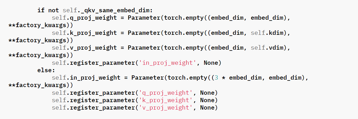
代码中，嵌入层向量还需要经过q_proj_weight 、k_proj_weight 、v_proj_weight 后才给入到注意力计算，而本文的代码为了简单方便描述过程，直接计算了，下面是官网代码片段：

10. 何为QKV？

QKV即是注意力机制，重点是"注意力"，通过这种计算，可以讲更任务更重心的位置放在更关键的位置上。QK的组合是一种注意力选择，选择V中的重要特征。

QKV 注意力机制是通过计算查询（Query）与键（Key）之间的相似度来衡量不同单词之间的关联程度，进而确定每个单词对于其他单词的重要性，从而实现更精准的信息提取和编码。具体来说，QKV 注意力机制的有效性源自于以下几个方面：

投影矩阵的作用：首先，通过投影矩阵将原始的词向量映射到 Q、K、V 空间。这个映射过程有助于模型学习到不同维度上的语义信息，并且使得后续计算更具有表征性。这样做的好处在于，通过对输入进行线性变换，模型可以更灵活地调整每个词在不同空间的表示，从而更好地匹配和捕捉语义关系。
相似度计算：Q 和 K 之间的点积运算衡量了查询与键之间的相似度。这一步是注意力机制的关键，因为它决定了不同单词之间的关联程度。点积计算的结果越大，表示两个向量之间的相关性越高，因此在后续的 Softmax 函数中会得到更高的权重，从而更多地关注相关性较高的单词。
归一化：Softmax 函数对相似度进行归一化，将其转化为概率分布。这一步使得模型能够更加专注于重要的信息，同时抑制不相关信息的影响。通过将相似度转化为概率分布，模型可以更好地选择与当前查询最相关的信息，提高了信息的利用效率。
加权平均：最后，将归一化后的相似度作为权重，对值向量 V 进行加权平均。这一步实际上是根据查询和键之间的相似度来调整值的重要性，从而得到最终的输出。这样做的好处在于，模型能够在保留原始信息的基础上，更好地关注与当前查询相关的信息，实现了信息的精准提取和利用。

总的来说，QKV 注意力机制通过将输入进行线性变换，并通过点积相似度计算、归一化和加权平均等步骤，实现了对不同单词之间关联程度的准确度量和精细控制，从而有效地提升了模型的表征能力和性能。

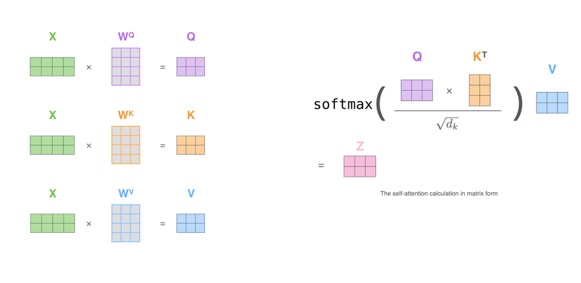
视频里有讲计算过程。不同单词的词向量先被QKV投影矩阵W投影到qkv：

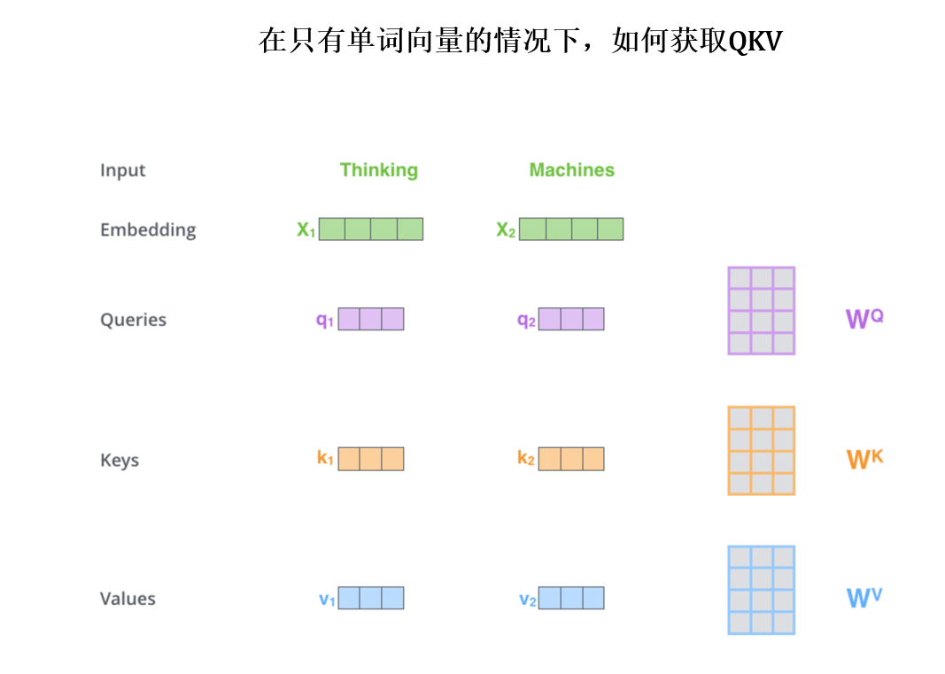
那么计算注意力的过程就如下图片：
Attention ( Q , K , V ) = softmax ( Q K T d k ) V \text{Attention}(Q, K, V) = \text{softmax}\left(\frac{QK^T}{\sqrt{d_k}}\right)V Attention(Q,K,V)=softmax(dk QKT)V

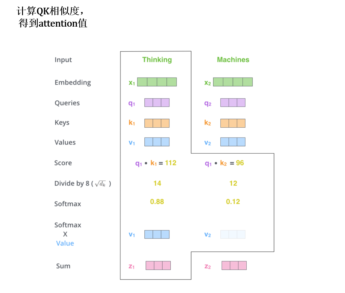
也就是这个图：

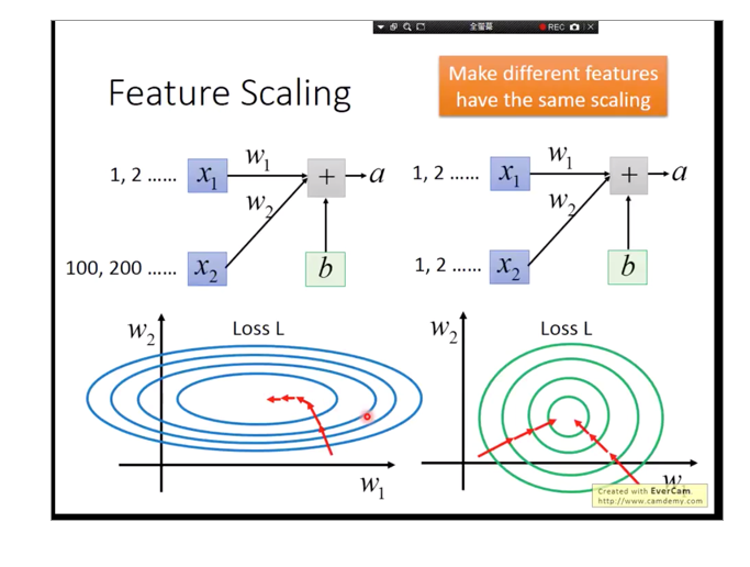
11. 为何不是BN？

使用的是Layer Normalization ，而不是BN，为何？

Layer Normalization (LN) 是一种深度学习中的归一化技术，它用于将神经网络中的每个层的输入进行归一化处理。Layer Normalization 将每个样本的输入进行归一化，即对每个样本在每个特征维度上进行归一化，而不是像 BN 那样对每个特征维度在一个 batch 中进行归一化。

LN 的计算方式如下：

对于一个输入向量 ( x = [x_1, x_2, ..., x_n] )，计算均值 ( \mu ) 和方差 ( \sigma^2 )：
μ = 1 n ∑ i = 1 n x i \mu = \frac{1}{n} \sum_{i=1}^{n} x_i μ=n1i=1∑nxi
σ 2 = 1 n ∑ i = 1 n ( x i − μ ) 2 \sigma^2 = \frac{1}{n} \sum_{i=1}^{n} (x_i - \mu)^2 σ2=n1i=1∑n(xi−μ)2
对输入向量 ( x ) 进行归一化：
x i ^ = x i − μ σ 2 + ϵ \hat{x_i} = \frac{x_i - \mu}{\sqrt{\sigma^2 + \epsilon}} xi^=σ2+ϵ xi−μ

其中，( \epsilon ) 是一个很小的常数，避免分母为零。
将归一化后的向量 ( \hat{x} ) 通过缩放参数 ( \gamma ) 和偏移参数 ( \beta ) 进行线性变换：
y i = γ x i ^ + β y_i = \gamma \hat{x_i} + \beta yi=γxi^+β

这样，LN 会保留每个样本的独立特性，而不会像 BN 那样受到 batch 中其他样本的影响。

BN受到其他样本影响太大，可以比作这个图：

12. RNN的梯度消失是指什么？

RNN的梯度消失和其他模型的梯度消失有本质差别：

一般意义的梯度消失是指在神经网络的反向传播过程中，梯度在经过多个层次传播时逐渐变小，并最终接近于零的现象。这导致在更新网络参数时，某些层的参数几乎没有更新，从而使得这些层无法有效地学习到输入数据的特征。【关键词，层数影响】

对于其他类型的神经网络，比如深度前馈神经网络（Feedforward Neural Networks），梯度消失通常与网络的深度有关。在深度神经网络中，梯度需要通过多个层次反向传播，而在每一层中都可能受到梯度逐渐衰减的影响，特别是在使用一些传统的激活函数（如 sigmoid 或 tanh）时更容易出现这种情况。

相比之下，RNN 的梯度消失问题与其循环结构和时间依赖关系密切相关。由于 RNN 的循环连接使得网络能够处理序列数据，并在每个时间步都与前一个时间步相关联，梯度需要在时间维度上传播。因此，RNN 的梯度消失问题通常与序列长度、时间步数以及网络架构中的循环连接有关。【关键词，多个时间步数迭代，多次迭代后的影响】

如何降低RNN的梯度消失

长短期记忆网络（LSTM）和门控循环单元（GRU）是为了解决 RNN 中的梯度消失问题而设计的。它们通过引入门控机制，可以选择性地记忆或遗忘先前的信息，从而更好地捕捉长期依赖关系。下面我将简要介绍它们的门控机制和公式。

长短期记忆网络（LSTM）

LSTM 引入了三个门：输入门（input gate）、遗忘门（forget gate）和输出门（output gate）。这些门控制着信息的流动，从而允许网络在处理序列数据时选择性地记忆或遗忘信息。

输入门：
i t = σ ( W i ⋅ [ h t − 1 , x t ] + b i ) i_t = \sigma(W_i \cdot [h_{t-1}, x_t] + b_i) it=σ(Wi⋅[ht−1,xt]+bi)
遗忘门：
f t = σ ( W f ⋅ [ h t − 1 , x t ] + b f ) f_t = \sigma(W_f \cdot [h_{t-1}, x_t] + b_f) ft=σ(Wf⋅[ht−1,xt]+bf)
输出门：
o t = σ ( W o ⋅ [ h t − 1 , x t ] + b o ) o_t = \sigma(W_o \cdot [h_{t-1}, x_t] + b_o) ot=σ(Wo⋅[ht−1,xt]+bo)
细胞状态更新：
c t = f t ⊙ c t − 1 + i t ⊙ tanh ( W c ⋅ [ h t − 1 , x t ] + b c ) c_t = f_t \odot c_{t-1} + i_t \odot \text{tanh}(W_c \cdot [h_{t-1}, x_t] + b_c) ct=ft⊙ct−1+it⊙tanh(Wc⋅[ht−1,xt]+bc)
隐藏状态更新：
h t = o t ⊙ tanh ( c t ) h_t = o_t \odot \text{tanh}(c_t) ht=ot⊙tanh(ct)

其中，(\sigma) 是 Sigmoid 函数，(\odot) 表示逐元素相乘，(W) 和 (b) 是模型的权重和偏置，([h_{t-1}, x_t]) 是上一时间步的隐藏状态和当前时间步的输入的连接，(\text{tanh}) 是双曲正切函数。

门控循环单元（GRU）

GRU 也具有类似的门控机制，但它将输入门和遗忘门合并为一个单一的更新门（update gate），并引入了重置门（reset gate）来控制历史信息的保留。GRU 的公式如下：

更新门：
z t = σ ( W z ⋅ [ h t − 1 , x t ] + b z ) z_t = \sigma(W_z \cdot [h_{t-1}, x_t] + b_z) zt=σ(Wz⋅[ht−1,xt]+bz)
重置门：
r t = σ ( W r ⋅ [ h t − 1 , x t ] + b r ) r_t = \sigma(W_r \cdot [h_{t-1}, x_t] + b_r) rt=σ(Wr⋅[ht−1,xt]+br)
更新隐藏状态：
h t = ( 1 − z t ) ⊙ h t − 1 + z t ⊙ tanh ( W h ⋅ [ r t ⊙ h t − 1 , x t ] + b h ) h_t = (1 - z_t) \odot h_{t-1} + z_t \odot \text{tanh}(W_h \cdot [r_t \odot h_{t-1}, x_t] + b_h) ht=(1−zt)⊙ht−1+zt⊙tanh(Wh⋅[rt⊙ht−1,xt]+bh)

其中，(z_t) 是更新门，(r_t) 是重置门，(W) 和 (b) 是模型的权重和偏置，([h_{t-1}, x_t]) 是上一时间步的隐藏状态和当前时间步的输入的连接，(\odot) 表示逐元素相乘，(\sigma) 是 Sigmoid 函数，(\text{tanh}) 是双曲正切函数。

通过这些门控机制，LSTM 和 GRU 能够更好地控制信息的流动，并且减轻了梯度消失问题，使得网络能够更有效地捕捉长期依赖关系。