基于RNN的股票市场时间序列预测(Python)

Step 1: Loading the data

import numpy as np
import pandas as pd
import matplotlib.pyplot as plt


import torch.nn as nn
import torch
from torch.autograd import Variable
from torch.utils.data import Dataset, DataLoader
# Importing the training set
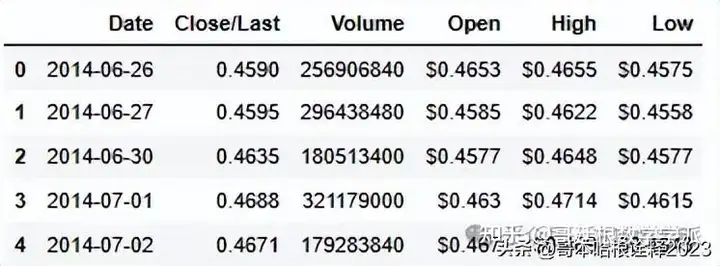
dataset = pd.read_csv('HistoricalData_1719412320530.csv')
dataset.head(10)

dataset.info()
<class 'pandas.core.frame.DataFrame'>
RangeIndex: 2516 entries, 0 to 2515
Data columns (total 6 columns):
 #   Column      Non-Null Count  Dtype 
---  ------      --------------  ----- 
 0   Date        2516 non-null   object
 1   Close/Last  2516 non-null   object
 2   Volume      2516 non-null   int64 
 3   Open        2516 non-null   object
 4   High        2516 non-null   object
 5   Low         2516 non-null   object
dtypes: int64(1), object(5)
memory usage: 118.1+ KB
# change time order


dataset['Date'] = pd.to_datetime(dataset['Date'], format='%m/%d/%Y')


# Sort the DataFrame in ascending order
dataset = dataset.sort_values(by='Date', ascending=True)


# Reset index if necessary
dataset = dataset.reset_index(drop=True)
dataset.head(5)

dataset['Close/Last'] = dataset['Close/Last'].str.replace('$', '').astype(float)
dataset.head(5)

dataset_cl = dataset['Close/Last'].values
# Feature Scaling
from sklearn.preprocessing import MinMaxScaler


sc = MinMaxScaler(feature_range = (0, 1))


# scale the data
dataset_cl = dataset_cl.reshape(dataset_cl.shape[0], 1)
dataset_cl = sc.fit_transform(dataset_cl)
dataset_cl
array([[2.91505500e-04],
       [2.95204809e-04],
       [3.24799276e-04],
       ...,
       [9.33338463e-01],
       [8.70746165e-01],
       [9.29787127e-01]])

Step 2: Cutting time series into sequences (Sliding Window)

input_size = 7


# Create a function to process the data into 7 day look back slices
# lb is window size
def processData(data, lb):
    X, y = [], [] # X is input vector, Y is output vector
    for i in range(len(data) - lb - 1):
        X.append(data[i: (i + lb), 0])
        y.append(data[(i + lb), 0])
    return np.array(X), np.array(y)


X, y = processData(dataset_cl, input_size)

Step 3: Split training and testing sets

X_train, X_test = X[:int(X.shape[0]*0.80)], X[int(X.shape[0]*0.80):]
y_train, y_test = y[:int(y.shape[0]*0.80)], y[int(y.shape[0]*0.80):]
print(X_train.shape[0])
print(X_test.shape[0])
print(y_train.shape[0])
print(y_test.shape[0])


# reshaping
X_train = np.reshape(X_train, (X_train.shape[0], 1, X_train.shape[1]))
X_test = np.reshape(X_test, (X_test.shape[0], 1, X_test.shape[1]))
2006
502
2006
502

Step 4: Build and run an RNN regression model

class RNN(nn.Module):
    def __init__(self, i_size, h_size, n_layers, o_size, dropout=0.1, bidirectional=False):
        super().__init__()
        # super(RNN, self).__init__()


        self.num_directions = bidirectional + 1


        # LSTM module
        self.rnn = nn.LSTM(
            input_size = i_size,
            hidden_size = h_size,
            num_layers = n_layers,
            dropout = dropout,
            bidirectional = bidirectional
        )


        # self.relu = nn.ReLU()


        # Output layer
        self.out = nn.Linear(h_size, o_size)


    def forward(self, x, h_state):
      # r_out contains the LSTM output at each time step, and hidden_state
      # contains the hidden and cell states after processing the entire sequence.
        r_out, hidden_state = self.rnn(x, h_state)


        hidden_size = hidden_state[-1].size(-1)


        # Convert dimension of r_out (-1 denotes it depends on other parameters)
        r_out = r_out.view(-1, self.num_directions, hidden_size)


        # r_out = self.relu(r_out)


        outs = self.out(r_out)


        return outs, hidden_state
# Global setting
INPUT_SIZE = input_size # LSTM input size


HIDDEN_SIZE = 256


NUM_LAYERS = 3 # LSTM 'stack' layer


OUTPUT_SIZE = 1




# Hyper parameters
learning_rate = 0.001
num_epochs = 300


rnn = RNN(INPUT_SIZE, HIDDEN_SIZE, NUM_LAYERS, OUTPUT_SIZE, bidirectional=False)
rnn.cuda()


optimiser = torch.optim.Adam(rnn.parameters(), lr=learning_rate)
criterion = nn.MSELoss()


hidden_state = None
rnn
RNN(
  (rnn): LSTM(7, 256, num_layers=3, dropout=0.1)
  (out): Linear(in_features=256, out_features=1, bias=True)
)
history = [] # save loss in each epoch
# .cuda() copies element to the GPU memory
X_test_cuda = torch.tensor(X_test).float().cuda()
y_test_cuda = torch.tensor(y_test).float().cuda()


# Use all the data in one batch
inputs_cuda = torch.tensor(X_train).float().cuda()
labels_cuda = torch.tensor(y_train).float().cuda()


# training
for epoch in range(num_epochs):


    # Train mode
    rnn.train()


    output, _ = rnn(inputs_cuda, hidden_state)
    # print(output.size())


    loss = criterion(output[:,0,:].view(-1), labels_cuda)
    optimiser.zero_grad()
    loss.backward()   # back propagation
    optimiser.step()   # update the parameters


    if epoch % 20 == 0:
        # Convert train mode to evaluation mode (disable dropout)
        rnn.eval()


        test_output, _ = rnn(X_test_cuda, hidden_state)
        test_loss = criterion(test_output.view(-1), y_test_cuda)
        print('epoch {}, loss {}, eval loss {}'.format(epoch, loss.item(), test_loss.item()))
    else:
        print('epoch {}, loss {}'.format(epoch, loss.item()))
    history.append(loss.item())
# iterate over all the learnable parameters in the model, which include the
# weights and biases of all layers in the model
# (both the LSTM layers and the final linear layer)
for param in rnn.parameters():
    print(param.data)

Step 5: Checking model performance

plt.plot(history)
# dplt.plot(history.history['val_loss'])

# X_train_X_test = np.concatenate((X_train, X_test),axis=0)
# hidden_state = None
rnn.eval()
# test_inputs = torch.tensor(X_test).float().cuda()
test_predict, _ = rnn(X_test_cuda, hidden_state)
test_predict_cpu = test_predict.cpu().detach().numpy()
plt.plot(sc.inverse_transform(y_test.reshape(-1,1)))
plt.plot(sc.inverse_transform(test_predict_cpu.reshape(-1,1)))
plt.legend(['y_test','test_predict_cpu'], loc='center left', bbox_to_anchor=(1, 0.5))

# plot original data
plt.plot(sc.inverse_transform(y.reshape(-1,1)), color='k')


# train_inputs = torch.tensor(X_train).float().cuda()
train_pred, hidden_state = rnn(inputs_cuda, None)
train_pred_cpu = train_pred.cpu().detach().numpy()


# use hidden state from previous training data
test_predict, _ = rnn(X_test_cuda, hidden_state)
test_predict_cpu = test_predict.cpu().detach().numpy()


# plt.plot(scl.inverse_transform(y_test.reshape(-1,1)))
split_pt = int(X.shape[0] * 0.80) + 7 # window_size
plt.plot(np.arange(7, split_pt, 1), sc.inverse_transform(train_pred_cpu.reshape(-1,1)), color='b')
plt.plot(np.arange(split_pt, split_pt + len(test_predict_cpu), 1), sc.inverse_transform(test_predict_cpu.reshape(-1,1)), color='r')


# pretty up graph
plt.xlabel('day')
plt.ylabel('price of Nvidia stock')
plt.legend(['original series','training fit','testing fit'], loc='center left', bbox_to_anchor=(1, 0.5))
plt.show()

MMSE = np.sum((test_predict_cpu.reshape(1,X_test.shape[0])-y[2006:])**2)/X_test.shape[0]
print(MMSE)
0.0018420128176938062



担任《Mechanical System and Signal Processing》审稿专家，担任《中国电机工程学报》，《控制与决策》等EI期刊审稿专家，擅长领域：现代信号处理，机器学习，深度学习，数字孪生，时间序列分析，设备缺陷检测、设备异常检测、设备智能故障诊断与健康管理PHM等。

 
知乎学术咨询：https://www.zhihu.com/consult/people/792359672131756032?isMe=1