【深度学习入门项目】基于支持向量机的手写数字识别

导入必要的包

numpy: 这个库是Python中常用的数学计算库。在这个项目中，我使用numpy来处理图像数据，将图像数据转换为一维向量，以便进行模型训练和测试。

matplotlib: 这个库是Python中常用的绘图库。在这个项目中，我使用matplotlib来显示一些手写数字图像样本以及测试样本和它们的预测结果。

sklearn: 这个库是Python中常用的机器学习库，提供了许多机器学习算法和工具。在这个项目中，使用sklearn来加载手写数字数据集、将数据集分为训练集和测试集、创建SVM分类器、进行模型训练和测试，并评估模型性能。

java 复制代码

import numpy as np
import matplotlib.pyplot as plt
from sklearn import datasets
from sklearn.model_selection import train_test_split
from sklearn.svm import SVC
from sklearn.metrics import confusion_matrix

1. 数据集

使用Scikit-Learn库自带的手写数字数据集（digits dataset）。该数据集包含8x8像素的手写数字图像，共有10个类别（数字0到9），每个类别有约180个样本，总共大约有1797个样本。

并且通过以下代码展示数据集中的基本信息

java 复制代码

# 加载手写数字数据集
digits = datasets.load_digits()

# 显示数据集基本信息
print("数据集基本信息:")
print("样本数量: {}".format(len(digits.images)))
print("图像大小: {}".format(digits.images[0].shape))

数据集基本信息:

样本数量: 1797

图像大小: (8, 8)\

java 复制代码

# 显示一些样本图像
fig, axes = plt.subplots(4, 4, figsize=(8, 8),
                         subplot_kw={'xticks':[], 'yticks':[]},
                         gridspec_kw=dict(hspace=0.1, wspace=0.1))

for i, ax in enumerate(axes.flat):
    ax.imshow(digits.images[i], cmap='binary', interpolation='nearest')
    ax.text(0.05, 0.05, str(digits.target[i]),
            transform=ax.transAxes, color='green' if (digits.target[i]==digits.target[0]) else 'black')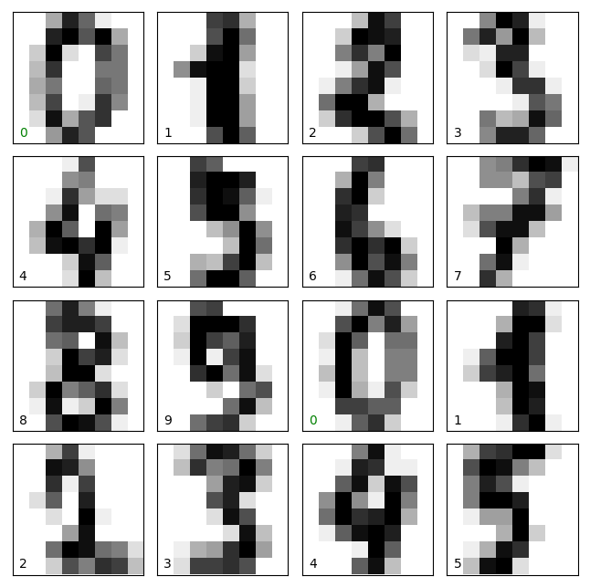

2. 数据处理

由于数据为8×8的图像数据，因此每个图像包含64个像素值。如果不将图像数据转换为一维向量，算法无法处理直接矩阵的数据。我们需要将数据转化为一维向量，来让SVM能够处理数据。这个过程通过numpy库中的reshape()函数实现。

同时由于是机器学习项目，我们需要划分训练集和测试集，通过使用sklearn库中的train_test_split函数来随机划分数据集为训练集和测试集。具体地，我将手写数字数据集中的样本随机划分为训练集和测试集，其中训练集占总样本数的70%，测试集占30%。这个划分比例可以根据实际情况进行调整。

java 复制代码

# 将图像数据转换为一维向量
X = digits.images.reshape((len(digits.images), -1))
y = digits.target

# 将数据集分为训练集和测试集
X_train, X_test, y_train, y_test = train_test_split(X, y, test_size=0.3)

3. 训练过程

使用sklearn库中的SVC()函数创建SVM分类器，并指定超参数。在这个项目中，参数是gamma=0.001。在实际使用中，我们可以多次调整参数，结合损失函数的变化，以寻得最优的参数。或者也可以直接使用默认的参数设置，即clf = SVC。

训练模型：使用SVM分类器对训练集进行训练，通过调用fit()方法实现。

预测结果：使用训练好的SVM分类器对测试集进行预测，通过调用predict()方法实现。

java 复制代码

# 创建SVM分类器
clf = SVC(gamma=0.001)

# 训练分类器
clf.fit(X_train, y_train)

# 测试分类器
y_pred = clf.predict(X_test)

4. 输出结果

首先是评估模型的性能，使用sklearn库中的confusion_matrix()函数计算模型的混淆矩阵，混淆矩阵的行表示实际标签，列表示预测标签，每个元素表示实际标签为该行所对应的数字，而分类器预测为该列所对应的数字的样本数。混淆矩阵可以比较直观的展示该项目中分类错误的个数，并根据混淆矩阵计算出模型的准确率、精确率、召回率和F1分数等指标。

java 复制代码

# 输出混淆矩阵和准确率
cm = confusion_matrix(y_test, y_pred)
print("混淆矩阵:")
print(cm)

accuracy = clf.score(X_test, y_test)
print("准确率: {:.2f}%".format(accuracy * 100))

# 显示一些测试样本和其预测结果
fig, axes = plt.subplots(4, 4, figsize=(8, 8),
                         subplot_kw={'xticks':[], 'yticks':[]},
                         gridspec_kw=dict(hspace=0.1, wspace=0.1))

for i, ax in enumerate(axes.flat):
    ax.imshow(X_test[i].reshape(8,8), cmap='binary', interpolation='nearest')
    ax.text(0.05, 0.05, str(y_pred[i]),
            transform=ax.transAxes,
            color='green' if (y_pred[i]==y_test[i]) else 'red')

plt.show()

混淆矩阵:
$\[56 0 0 0 0 0 0 0 0 0$ $0 57 0 0 0 0 0 0 0 0$ $0 0 44 0 0 0 0 0 0 0$ $0 0 0 60 0 0 0 0 0 0$ $0 0 0 0 70 0 0 0 0 0$ $0 0 0 0 0 56 1 0 0 0$ $0 0 0 0 0 0 48 0 0 0$ $0 0 0 0 0 0 0 55 0 1$ $0 1 0 0 0 0 0 0 49 0$ $0 0 0 0 0 0 0 1 0 41\]$
准确率: 99.26%

完整代码

java 复制代码

import numpy as np
import matplotlib.pyplot as plt
from sklearn import datasets
from sklearn.model_selection import train_test_split
from sklearn.svm import SVC
from sklearn.metrics import confusion_matrix

# 加载手写数字数据集
digits = datasets.load_digits()

# 显示数据集基本信息
print("数据集基本信息:")
print("样本数量: {}".format(len(digits.images)))
print("图像大小: {}".format(digits.images[0].shape))

# 显示一些样本图像
fig, axes = plt.subplots(4, 4, figsize=(8, 8),
                         subplot_kw={'xticks':[], 'yticks':[]},
                         gridspec_kw=dict(hspace=0.1, wspace=0.1))

for i, ax in enumerate(axes.flat):
    ax.imshow(digits.images[i], cmap='binary', interpolation='nearest')
    ax.text(0.05, 0.05, str(digits.target[i]),
            transform=ax.transAxes, color='green' if (digits.target[i]==digits.target[0]) else 'black')

# 将图像数据转换为一维向量
X = digits.images.reshape((len(digits.images), -1))
y = digits.target

# 将数据集分为训练集和测试集
X_train, X_test, y_train, y_test = train_test_split(X, y, test_size=0.3)

# 创建SVM分类器
clf = SVC(gamma=0.001)

# 训练分类器
clf.fit(X_train, y_train)

# 测试分类器
y_pred = clf.predict(X_test)

# 输出混淆矩阵和准确率
cm = confusion_matrix(y_test, y_pred)
print("混淆矩阵:")
print(cm)

accuracy = clf.score(X_test, y_test)
print("准确率: {:.2f}%".format(accuracy * 100))

# 显示一些测试样本和其预测结果
fig, axes = plt.subplots(4, 4, figsize=(8, 8),
                         subplot_kw={'xticks':[], 'yticks':[]},
                         gridspec_kw=dict(hspace=0.1, wspace=0.1))

for i, ax in enumerate(axes.flat):
    ax.imshow(X_test[i].reshape(8,8), cmap='binary', interpolation='nearest')
    ax.text(0.05, 0.05, str(y_pred[i]),
            transform=ax.transAxes,
            color='green' if (y_pred[i]==y_test[i]) else 'red')

plt.show()

【深度学习入门项目】基于支持向量机的手写数字识别

目录

导入必要的包

1. 数据集

2. 数据处理

3. 训练过程

4. 输出结果

完整代码