目录
前言
过采样(Oversampling)是指在数据处理或机器学习中,增加少数类样本的数量以平衡类别分布。常用于处理类别不平衡问题,通过复制少数类样本或生成新样本来提高模型对少数类的识别能力。
一、为什么使用过采样?
- 当不同类别的数据量不均衡时
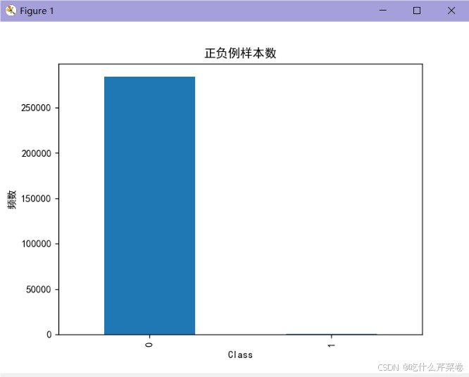
- 这会导致某一类别的正确率很低
- 这时可以使用过采样方法:
- 先分出训练集和测试集
- 使用过采样方法拟合类别少的数据
- 使两种类型的数据均衡
- 此时结果不同类别的正确率将会得到提高
二、代码实现
1.完整代码
python
import pandas as pd
import matplotlib.pyplot as plt
import numpy as np


# 可视化混淆矩阵
def cm_plot(y, yp):
    from sklearn.metrics import confusion_matrix
    import matplotlib.pyplot as plt

    cm = confusion_matrix(y, yp)
    plt.matshow(cm, cmap=plt.cm.Blues)
    plt.colorbar()
    for x in range(len(cm)):
        for y in range(len(cm)):
            plt.annotate(cm[x, y], xy=(y, x), horizontalalignment='center',
                         verticalalignment='center')
            plt.ylabel('True label')
            plt.xlabel('Predicted label')
    return plt


data = pd.read_csv("creditcard.csv")

# 数据标准化: Z标准化
from sklearn.preprocessing import StandardScaler  # 可对多列进行标准化

scaler = StandardScaler()
a = data[['Amount']]  # 取出来变成df数据 因为fit_transform()需要传入df数据
data['Amount'] = scaler.fit_transform(a)  # 对Amount列数据进行标准化
data = data.drop(['Time'], axis=1)  # 删除无用列

# 随机取数据 小数据集
from sklearn.model_selection import train_test_split

x = data.drop('Class', axis=1)
y = data.Class
x_w_train, x_w_test, y_w_train, y_w_test = \
    train_test_split(x, y, test_size=0.2, random_state=0)  # 随机取数据

"""过采样"""
from imblearn.over_sampling import SMOTE

oversampler = SMOTE(random_state=0)  # 随机种子 保证数据拟合效果
x_os, y_os = oversampler.fit_resample(x_w_train, y_w_train)  # 通过原始训练集的特征和标签数据人工拟合一份训练集和标签

# 绘制条形图 查看样本个数
plt.rcParams['font.sans-serif'] = ['SimHei']  # 设置字体
plt.rcParams['axes.unicode_minus'] = False  # 解决符号显示为方块的问题
labels_count = pd.value_counts(y_os)  # 统计0有多少个数据,1有多个数据
plt.title("正负例样本数")
plt.xlabel("类别")
plt.ylabel("频数")
labels_count.plot(kind='bar')  # 生成一个条形图,展示每个类别的样本数量。
plt.show()

x_os_train, x_os_test, y_os_train, y_os_test = \
    train_test_split(x_os, y_os, test_size=0.2, random_state=0)  # 随机取数据

# 交叉验证选择较优惩罚因子 λ
from sklearn.model_selection import cross_val_score  # 交叉验证的函数
from sklearn.linear_model import LogisticRegression

# k折交叉验证选择C参数
scores = []
c_param_range = [0.01, 0.1, 1, 10, 100]  # 待选C参数
for i in c_param_range:
    lr = LogisticRegression(C=i, penalty='l2', solver='lbfgs', max_iter=1000)  # 创建逻辑回归模型  lbfgs 拟牛顿法
    score = cross_val_score(lr, x_os_train, y_os_train, cv=8, scoring='recall')  # k折交叉验证 比较召回率
    score_mean = sum(score) / len(score)
    scores.append(score_mean)
    print(score_mean)

best_c = c_param_range[np.argmax(scores)]  # 寻找到scores中最大值的对应的C参数
print(f"最优惩罚因子为:{best_c}")

# 建立最优模型
lr = LogisticRegression(C=best_c, penalty='l2', max_iter=1000)
lr.fit(x_os_train, y_os_train)

# 绘制混淆矩阵
from sklearn import metrics

x_os_train_predicted = lr.predict(x_os_train)  # 训练集特征数据x的预测值
print(metrics.classification_report(y_os_train, x_os_train_predicted))  # 传入训练集真实的结果数据 与预测值组成矩阵

x_os_test_predicted = lr.predict(x_os_test)  # 训练集特征数据x的预测值
print(metrics.classification_report(y_os_test, x_os_test_predicted))  # 传入训练集真实的结果数据 与预测值组成矩阵

x_w_test_predicted = lr.predict(x_w_test)
print(metrics.classification_report(y_w_test, x_w_test_predicted))
2.数据预处理
- 导入数据
- 对特征进行标准化
- 随机取出训练集和测试集
python
import pandas as pd
import matplotlib.pyplot as plt
import numpy as np

data = pd.read_csv("creditcard.csv")

# 数据标准化: Z标准化
from sklearn.preprocessing import StandardScaler  # 可对多列进行标准化

scaler = StandardScaler()
a = data[['Amount']]  # 取出来变成df数据 因为fit_transform()需要传入df数据
data['Amount'] = scaler.fit_transform(a)  # 对Amount列数据进行标准化
data = data.drop(['Time'], axis=1)  # 删除无用列

# 随机取数据 小数据集
from sklearn.model_selection import train_test_split

x = data.drop('Class', axis=1)
y = data.Class
x_w_train, x_w_test, y_w_train, y_w_test = \
    train_test_split(x, y, test_size=0.2, random_state=0)  # 随机取数据
3.进行过采样
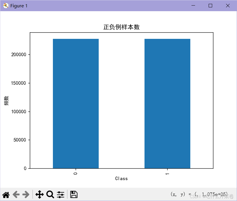
- 使用over_sampling 里的SMOTE模块
- 对训练集数据进行过采样,拟合数据
- 查看拟合之后的数据集
- 从该数据集中分出训练集和测试集
python
"""过采样"""
from imblearn.over_sampling import SMOTE

oversampler = SMOTE(random_state=0)  # 随机种子 保证数据拟合效果
x_os, y_os = oversampler.fit_resample(x_w_train, y_w_train)  # 通过原始训练集的特征和标签数据人工拟合一份训练集和标签

# 绘制条形图 查看样本个数
plt.rcParams['font.sans-serif'] = ['SimHei']  # 设置字体
plt.rcParams['axes.unicode_minus'] = False  # 解决符号显示为方块的问题
labels_count = pd.value_counts(y_os)  # 统计0有多少个数据,1有多个数据
plt.title("正负例样本数")
plt.xlabel("类别")
plt.ylabel("频数")
labels_count.plot(kind='bar')  # 生成一个条形图,展示每个类别的样本数量。
plt.show()

x_os_train, x_os_test, y_os_train, y_os_test = \
    train_test_split(x_os, y_os, test_size=0.2, random_state=0)  # 随机取数据
输出:

4.建立模型
- 使用k折交叉验证法选出最佳的C参数
- 训练所使用的数据是从拟合数据里取出来的训练集
- 建立最优模型
python
# 交叉验证选择较优惩罚因子 λ
from sklearn.model_selection import cross_val_score  # 交叉验证的函数
from sklearn.linear_model import LogisticRegression

# k折交叉验证选择C参数
scores = []
c_param_range = [0.01, 0.1, 1, 10, 100]  # 待选C参数
for i in c_param_range:
    lr = LogisticRegression(C=i, penalty='l2', solver='lbfgs', max_iter=1000)  # 创建逻辑回归模型  lbfgs 拟牛顿法
    score = cross_val_score(lr, x_os_train, y_os_train, cv=8, scoring='recall')  # k折交叉验证 比较召回率
    score_mean = sum(score) / len(score)
    scores.append(score_mean)
    print(score_mean)

best_c = c_param_range[np.argmax(scores)]  # 寻找到scores中最大值的对应的C参数
print(f"最优惩罚因子为:{best_c}")

# 建立最优模型
lr = LogisticRegression(C=best_c, penalty='l2', max_iter=1000)
lr.fit(x_os_train, y_os_train)
输出:
python
0.9096726221315528
0.9106337846987276
0.9109523409608787
0.9110237415273612
0.9110182489533213
最优惩罚因子为:10
5.绘制混淆矩阵
- 分别使用原始数据里取出来的测试集,拟合数据里取出来的训练集和测试集进行混淆矩阵的绘制
python
# 绘制混淆矩阵
from sklearn import metrics

x_os_train_predicted = lr.predict(x_os_train)  # 训练集特征数据x的预测值
print(metrics.classification_report(y_os_train, x_os_train_predicted))  # 传入训练集真实的结果数据 与预测值组成矩阵

x_os_test_predicted = lr.predict(x_os_test)  # 训练集特征数据x的预测值
print(metrics.classification_report(y_os_test, x_os_test_predicted))  # 传入训练集真实的结果数据 与预测值组成矩阵

x_w_test_predicted = lr.predict(x_w_test)
print(metrics.classification_report(y_w_test, x_w_test_predicted))
输出:
python
precision recall f1-score support
0 0.92 0.98 0.94 181855
1 0.97 0.91 0.94 182071
accuracy 0.94 363926
macro avg 0.94 0.94 0.94 363926
weighted avg 0.94 0.94 0.94 363926
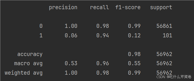
precision recall f1-score support
0 0.92 0.98 0.95 45599
1 0.97 0.91 0.94 45383
accuracy 0.94 90982
macro avg 0.95 0.94 0.94 90982
weighted avg 0.94 0.94 0.94 90982
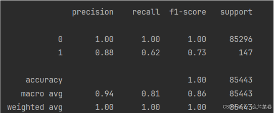
precision recall f1-score support
0 1.00 0.98 0.99 56861
1 0.06 0.94 0.12 101
accuracy 0.98 56962
macro avg 0.53 0.96 0.55 56962
weighted avg 1.00 0.98 0.99 56962总结
过采样适合不同类别数据不均衡的情况,下采样虽然也适合,但是一般情况下过采样要更加优秀