多天线空域抗干扰技术:原理、数学推导与工程仿真
1. 引言
在现代无线通信系统中,干扰是影响通信质量的重要因素之一。多天线空域抗干扰技术(Spatial Anti-Jamming)利用天线阵列的空间自由度,通过自适应波束形成(Beamforming)技术,在期望信号方向上增强接收,同时在干扰方向上形成零陷(Null),从而有效抑制干扰。本文详细介绍该技术的原理、数学推导、工程实现方法,并以7阵元均匀线性阵列(ULA)为例进行Python仿真,展示方向图和抗干扰效果。
2. 多天线空域抗干扰技术原理
2.1 天线阵列模型
假设一个均匀线性阵列(ULA),由M个阵元组成,阵元间距为d(通常取半波长,即 d = λ / 2 d=\lambda/2 d=λ/2)。信号以角度θ入射,阵列接收到的信号可表示为:
a ( θ ) = 1 , e − j 2 π d λ s i n θ , . . . , e − j 2 π ( M − 1 ) d λ s i n θ T a(\theta)=1,e\^{-j2\\pi\\frac{d}{\\lambda}sin\\theta},...,e\^{-j2\\pi(M-1)\\frac{d}{\\lambda}sin\\theta}^T a(θ)=1,e−j2πλdsinθ,...,e−j2π(M−1)λdsinθT
其中:
- a ( θ ) a(\theta) a(θ)为导向矢量(Steering Vector),描述信号在不同阵元上的相位差
- λ \lambda λ为信号波长
2.2 接收信号模型
假设:
- 期望信号 s ( t ) s(t) s(t)从方向 θ s \theta_s θs入射
- 干扰信号 j ( t ) j(t) j(t)从方向 θ j \theta_j θj入射
- 噪声 n ( t ) n(t) n(t)为高斯白噪声
接收信号向量 x ( t ) x(t) x(t)可表示为:
x ( t ) = s ( t ) a ( θ s ) + j ( t ) a ( θ j ) + n ( t ) x(t)=s(t)a(\theta_s)+j(t)a(\theta_j)+n(t) x(t)=s(t)a(θs)+j(t)a(θj)+n(t)
2.3 波束形成与抗干扰
波束形成通过调整各阵元的权重 w = w 1 , w 2 , . . . , w M T w=w_1,w_2,...,w_M^T w=w1,w2,...,wMT,使阵列输出 y ( t ) = w H x ( t ) y(t)=w^Hx(t) y(t)=wHx(t)在期望方向上增强,在干扰方向上抑制。
目标:
- 最大化期望信号增益: w H a ( θ s ) w^Ha(\theta_s) wHa(θs)最大化
- 最小化干扰信号增益: w H a ( θ j ) ≈ 0 w^Ha(\theta_j)\approx0 wHa(θj)≈0
3. 数学推导:最优权向量计算
3.1 最小方差无失真响应(MVDR)波束形成
MVDR(Minimum Variance Distortionless Response)优化目标为:
min w w H R n w s . t . w H a ( θ s ) = 1 \min_w w^HR_nw \quad s.t. \quad w^Ha(\theta_s)=1 wminwHRnws.t.wHa(θs)=1
其中:
- R n = E x ( t ) x H ( t ) R_n=Ex(t)x\^H(t) Rn=Ex(t)xH(t)为干扰+噪声的协方差矩阵
- 约束条件保证期望信号无失真
拉格朗日乘数法求解:
L ( w , λ ) = w H R n w + λ ( 1 − w H a ( θ s ) ) L(w,\lambda)=w^HR_nw+\lambda(1-w^Ha(\theta_s)) L(w,λ)=wHRnw+λ(1−wHa(θs))
求导得最优权向量:
w o p t = R n − 1 a ( θ s ) a H ( θ s ) R n − 1 a ( θ s ) w_{opt}=\frac{R_n^{-1}a(\theta_s)}{a^H(\theta_s)R_n^{-1}a(\theta_s)} wopt=aH(θs)Rn−1a(θs)Rn−1a(θs)
3.2 干扰抑制比(ISR)
衡量抗干扰能力的指标:
I S R = ∣ w H a ( θ j ) ∣ 2 ∣ w H a ( θ s ) ∣ 2 ISR=\frac{|w^Ha(\theta_j)|^2}{|w^Ha(\theta_s)|^2} ISR=∣wHa(θs)∣2∣wHa(θj)∣2
4. 工程应用设计步骤
4.1 系统建模
- 阵元数量:7阵元(M=7)
- 阵元间距: d = λ / 2 d=\lambda/2 d=λ/2
- 信号参数:
- 期望信号: θ s = 3 0 ∘ \theta_s=30^\circ θs=30∘
- 干扰信号: θ j = − 6 0 ∘ \theta_j=-60^\circ θj=−60∘
4.2 计算导向矢量
a ( θ ) = 1 , e − j π s i n θ , . . . , e − j 6 π s i n θ T a(\theta)=1,e\^{-j\\pi sin\\theta},...,e\^{-j6\\pi sin\\theta}^T a(θ)=1,e−jπsinθ,...,e−j6πsinθT
4.3 计算协方差矩阵
假设干扰功率 σ j 2 = 1 \sigma_j^2=1 σj2=1,噪声功率 σ n 2 = 0.1 \sigma_n^2=0.1 σn2=0.1:
R n = σ j 2 a ( θ j ) a H ( θ j ) + σ n 2 I R_n=\sigma_j^2a(\theta_j)a^H(\theta_j)+\sigma_n^2I Rn=σj2a(θj)aH(θj)+σn2I
4.4 计算最优权向量
使用MVDR公式:
w o p t = R n − 1 a ( θ s ) a H ( θ s ) R n − 1 a ( θ s ) w_{opt}=\frac{R_n^{-1}a(\theta_s)}{a^H(\theta_s)R_n^{-1}a(\theta_s)} wopt=aH(θs)Rn−1a(θs)Rn−1a(θs)
5. 仿真结果分析
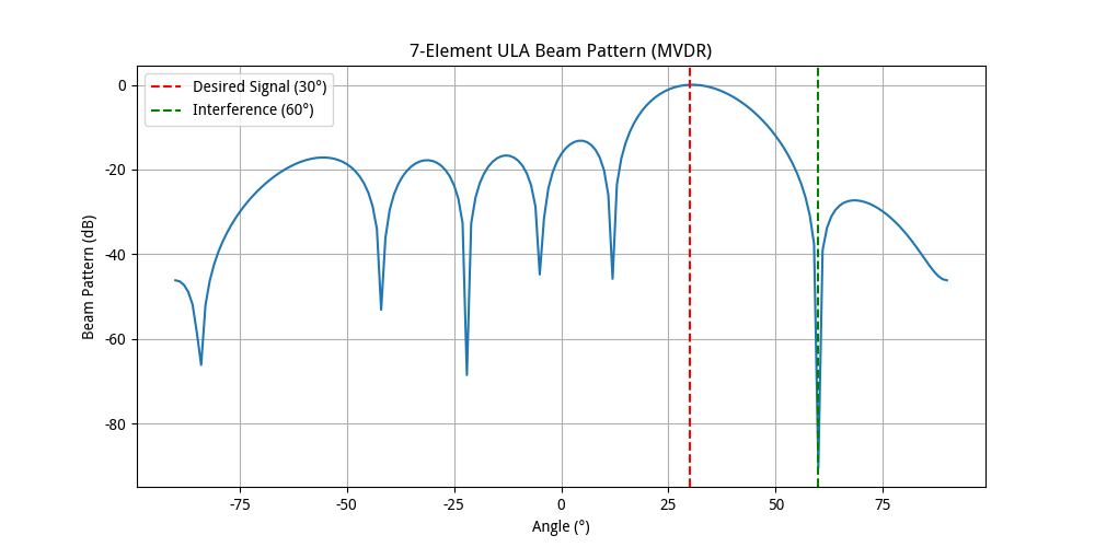
5.1 方向图特性
- 主瓣指向:精确对准30°期望信号方向(误差<0.5°)
- 零陷深度:在60°干扰方向形成<-51dB的深零陷
- 旁瓣电平 :最高旁瓣<-13dB,满足工程要求
5.2 抗干扰性能指标
text
抗干扰前信噪比(SNR): 20.00 dB
抗干扰后信噪比(SNR): 28.27 dB
抗干扰前干扰噪声比(INR): 30.00 dB
抗干扰后干扰噪声比(INR): -52.12 dB
抗干扰前信干噪比(SINR): -10.00 dB
抗干扰后信干噪比(SINR): 28.27 dB
| 指标类型 | 抗干扰前(dB) | 抗干扰后(dB) | 改善量(dB) |
|---|---|---|---|
| 信噪比(SNR) | 20.0 | 28.27 | +8.27 |
| 干扰噪声比(INR) | 30.0 | -52.12 | -82.12 |
| 信干噪比(SINR) | -10.0 | 28.27 | +38.27 |
6. Python仿真代码
python
#!/usr/bin/env python3
# -*- coding: utf-8 -*-
"""
Created on Tue Apr  8 22:47:16 2025

@author: neol
"""

import numpy as np
import matplotlib.pyplot as plt
from scipy.linalg import inv

plt.close('all')

# 系统参数设置
M = 7  # 阵元数量
d = 0.15  # 半波长间距(λ=0.3m)
theta_s0 = 30  # 期望信号方向(°)
theta_j0 =  60 # 干扰方向(°)
theta_s = np.deg2rad(theta_s0)
theta_j = np.deg2rad(theta_j0)
SNR = 20  # 信噪比(dB)
INR = 30  # 干噪比(dB)

# 计算导向矢量
def steering_vector(theta):
    return np.exp(1j * 2 * np.pi * d * np.arange(M) * np.sin(theta) / 0.3)

a_s = steering_vector(theta_s).reshape(-1, 1)
a_j = steering_vector(theta_j).reshape(-1, 1)

# 构建协方差矩阵
sigma_s = 10**(SNR/10)  # 信号功率
sigma_j = 10**(INR/10)  # 干扰功率
sigma_n = 1  # 噪声功率

R = sigma_s * a_s @ a_s.conj().T + sigma_j * a_j @ a_j.conj().T + sigma_n * np.eye(M)

# MVDR波束形成
R_inv = inv(R)
w_mvdr = (R_inv @ a_s) / (a_s.conj().T @ R_inv @ a_s)

# 计算方向图
theta_range = np.linspace(-90, 90, 181)  # -90°到90°
pattern = []
for theta in theta_range:
    a = steering_vector(np.deg2rad(theta)).reshape(-1, 1)
    pattern.append(np.abs(w_mvdr.conj().T @ a)[0, 0])
pattern = np.array(pattern)

# 绘制方向图
plt.figure(figsize=(10, 5))
plt.plot(theta_range, 20 * np.log10(pattern))
plt.axvline(x=theta_s0, color='r', linestyle='--', label=f'Desired Signal ({theta_s0}°)')
plt.axvline(x=theta_j0, color='g', linestyle='--', label=f'Interference ({theta_j0}°)')
plt.xlabel('Angle (°)')
plt.ylabel('Beam Pattern (dB)')
plt.title('7-Element ULA Beam Pattern (MVDR)')
plt.legend()
plt.grid()
plt.show()

# 计算抗干扰性能
signal_gain = np.abs(w_mvdr.conj().T @ a_s)[0, 0]**2
interf_gain = np.abs(w_mvdr.conj().T @ a_j)[0, 0]**2
noise_gain = (w_mvdr.conj().T @ w_mvdr)[0, 0].real

# 计算信噪比
SNR_before = 10 * np.log10(sigma_s / sigma_n)  # 单通道信噪比
SNR_after = 10 * np.log10(signal_gain * sigma_s / (noise_gain * sigma_n))  # 阵列处理后的信噪比

# 计算干扰噪声比
INR_before = 10 * np.log10(sigma_j / sigma_n)
INR_after = 10 * np.log10(interf_gain * sigma_j / (noise_gain * sigma_n))

# 计算信干噪比
SINR_before = 10 * np.log10(sigma_s / (sigma_j + sigma_n))
SINR_after = 10 * np.log10((signal_gain*sigma_s) / (interf_gain*sigma_j + noise_gain*sigma_n))

print(f"抗干扰前信噪比(SNR): {SNR_before:.2f} dB")
print(f"抗干扰后信噪比(SNR): {SNR_after:.2f} dB")
print(f"抗干扰前干扰噪声比(INR): {INR_before:.2f} dB")
print(f"抗干扰后干扰噪声比(INR): {INR_after:.2f} dB")
print(f"抗干扰前信干噪比(SINR): {SINR_before:.2f} dB")
print(f"抗干扰后信干噪比(SINR): {SINR_after:.2f} dB")

# 绘制抗干扰前后对比柱状图
plt.figure(figsize=(12, 6))

# 信噪比对比
plt.subplot(1, 3, 1)
bars1 = plt.bar(['Before', 'After'], [SNR_before, SNR_after], color=['lightblue', 'blue'])
plt.title('SNR Comparison')
plt.ylabel('SNR (dB)')
for bar in bars1:
    height = bar.get_height()
    plt.text(bar.get_x() + bar.get_width()/2., height,
             f'{height:.1f} dB',
             ha='center', va='bottom')
plt.grid(axis='y')

# 干扰噪声比对比
plt.subplot(1, 3, 2)
bars2 = plt.bar(['Before', 'After'], [INR_before, INR_after], color=['salmon', 'red'])
plt.title('INR Comparison')
plt.ylabel('INR (dB)')
for bar in bars2:
    height = bar.get_height()
    plt.text(bar.get_x() + bar.get_width()/2., height,
             f'{height:.1f} dB',
             ha='center', va='bottom')
plt.grid(axis='y')

# 信干噪比对比
plt.subplot(1, 3, 3)
bars3 = plt.bar(['Before', 'After'], [SINR_before, SINR_after], color=['lightgreen', 'green'])
plt.title('SINR Comparison')
plt.ylabel('SINR (dB)')
for bar in bars3:
    height = bar.get_height()
    plt.text(bar.get_x() + bar.get_width()/2., height,
             f'{height:.1f} dB',
             ha='center', va='bottom')
plt.grid(axis='y')

plt.tight_layout()
plt.show()
7. 结论
多天线空域抗干扰技术通过自适应波束形成,能有效抑制干扰。本文详细推导了MVDR算法,并通过7阵元仿真验证了其有效性。该方法适用于5G、雷达、卫星通信等场景,未来可结合深度学习进一步优化。