ReID/OSNet 算法模型量化转换实践

ReID 算法，全称是"行人再识别（Person Re-Identification）"算法，可应用于智能驾驶或智能机器人陪伴等领域。它的目标是在不同摄像头或不同时间拍摄的多张图像中，准确识别出是否为同一个人。本文以 ReID 中比较有名的 OSNet 模型为例，讲解如何在地平线计算平台量化该模型。

OSNet（Omni-Scale Network）是 行人再识别 任务中非常流行的一种深度学习架构，旨在高效提取行人图像中不同尺度的判别特征。

核心思想：Omni-Scale Feature Learning

OSNet 的核心思想是：在一个卷积块中同时捕捉多种尺度的信息，而不是像传统方法那样堆叠多个尺度层。

传统 ReID 网络可能在不同层捕捉不同尺度（如局部细节 vs 整体结构），但 OSNet 尝试在每一层同时捕捉小尺度和大尺度的信息。

osnet_ain_x1_0 是 OSNet 系列中性能较强的一个变体，其全称是：

OSNet-AIN-x1.0 ：Omni-Scale Network with Adaptive Instance Normalization（自适应实例归一化）

特点解析

1. 多尺度特征学习（OSNet 核心）

• OSBlock 模块引入多个不同感受野的卷积分支。
• 实现：局部细节与全局上下文同时建模。
• 相比传统 ResNet，有更强的判别性和更少的参数。

1. AIN：自适应实例****归一化

• Adaptive Instance Normalization 是一种可以调节风格的归一化方法，常用于领域自适应。

• 在 ReID 中，行人图像来自不同摄像头或环境，AIN 可以自适应不同图像风格，减轻 域偏移（domain shift） 的影响。

• 提升跨摄像头、跨数据集的识别能力。

一、源码导出 ONNX

1.1 克隆代码仓库

克隆代码仓库的 master 分支。

git clone https://github.com/KaiyangZhou/deep-person-reid.git

之后按照官方指导搭建好环境。

1.2 下载预训练权重

使用 Multi-source domain generalization 章节 osnet_ain_x1_0 的 MS+D+C->M 权重 osnet_ain_ms_d_c.pth.tar。

https://kaiyangzhou.github.io/deep-person-reid/MODEL_ZOO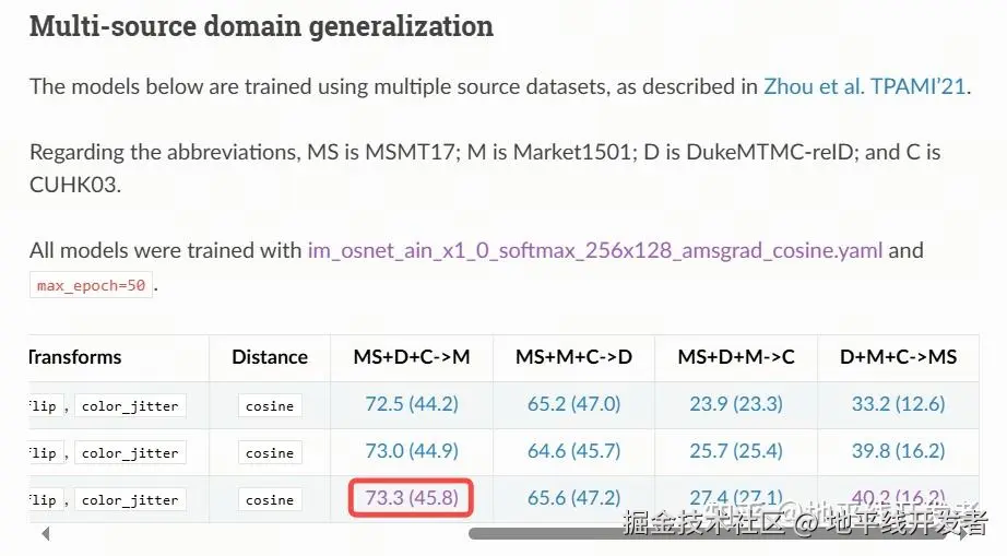

1.3 导出 onnx

将 osnet_ain_ms_d_c.pth.tar 权重文件存放到项目根目录，编写并运行 onnx 导出脚本。

import torch
from torchreid.utils.feature_extractor import FeatureExtractor

def export_onnx(model, im):
    f = 'osnet_ain_x1_0.onnx'
    torch.onnx.export(
        model.cpu(),
        im.cpu(),
        f,
        opset_version=11,
        do_constant_folding=True,
        input_names=['input'],
        output_names=['output']
    )
    return 0

if __name__ == "__main__":
    extractor = FeatureExtractor(
        model_name="osnet_ain_x1_0",
        model_path="./osnet_ain_ms_d_c.pth.tar",
        device=str('cpu')
    )
    im = torch.zeros(1, 3, 256, 128).to('cpu')
    export_onnx(extractor.model.eval(), im)

1.4 检查 onnx 和 pytorch 一致性

import onnx
import torch
import onnxruntime as ort
import numpy as np
from pathlib import Path
from torchreid.utils.feature_extractor import FeatureExtractor

def cosine_similarity(a, b):
    a = np.array(a)
    b = np.array(b)
    return np.dot(a, b) / (np.linalg.norm(a) * np.linalg.norm(b))

def max_difference(a, b):
    a = np.array(a).ravel()
    b = np.array(b).ravel()
    diff = np.abs(a - b)
    max_diff = np.max(diff)
    max_idx = np.argmax(diff)
    print(f"最大差值: {max_diff}，位置索引: {max_idx}")
    return max_diff, max_idx

if __name__ == "__main__":
    extractor = FeatureExtractor(
        model_name="osnet_ain_x1_0",
        model_path="./osnet_ain_ms_d_c.pth.tar",
        device=str('cpu')
    )
    im = torch.randn(1, 3, 256, 128).to('cpu')
    with torch.no_grad():
        pt_model = extractor.model.eval()
        output = pt_model(im)

    onnx_path = 'osnet_ain_x1_0.onnx'
    session = ort.InferenceSession(onnx_path, providers=['CPUExecutionProvider'])
    input_tensor =im.numpy()
    input_name = session.get_inputs()[0].name
    outputs = session.run(None, {input_name: input_tensor})
    output_tensor = outputs[0]

    print(cosine_similarity(output.numpy().reshape(-1), output_tensor.reshape(-1)))
    max_difference(output.numpy().reshape(-1), output_tensor.reshape(-1))

如果多次运行，相似度打印均为 1，且最大差值均在 e-5 以内，则可认为 onnx 和 pytorch 的输出保持一致。

二、PTQ 量化

2.1 生成校准数据

可以从官方数据集（Market-1501-v15.09.15）中选择数百张 jpg 图片用来生成校准数据。

在生成校准数据前，需要明确预处理参数，在源码 deep-person-reid-master/torchreid/data/transforms.py 中，可以得知训练时会将图片直接 resize 成模型输入尺寸，并使用 imagenet 数据集的标准归一化参数，即：

norm_mean = [0.485, 0.456, 0.406]
norm_std = [0.229, 0.224, 0.225]

且由归一化参数可知，模型训练时使用的色彩通道顺序是 rgb。

此时可以基于 horizon_model_convert_sample 提供的脚本生成校准数据，只需基于 02_preprocess.sh 和 preprocess.py 脚本做如下改动：

python3 ../../../data_preprocess.py \
  --src_dir ./market_1501_jpg \    # 从Market-1501-v15.09.15数据集挑选的jpg图片
  --dst_dir ./calib_data_rgb_f32 \ # 生成的校准数据文件夹
  --pic_ext .rgb \                 # 色彩通道顺序
  --read_mode opencv \             # 读图方式使用opencv
  --saved_data_type float32 \      # 校准数据的数据类型使用float32
  --cal_img_num 300                # 生成300份校准数据
from horizon_tc_ui.data.transformer import (
    BGR2RGBTransformer, HWC2CHWTransformer, ResizeTransformer)

def calibration_transformers():
    transformers = [
        ResizeTransformer(target_size=(256, 128)),  # 直接对图像做resize
        HWC2CHWTransformer(),                       # 从HWC更改为CHW
        BGR2RGBTransformer(data_format="CHW"),      # 将色彩通道顺序更改为RGB
    ]
    return transformers

由于归一化计算会集成到 PTQ 生成模型的预处理节点中，因此校准数据无需做归一化处理。

2.2 量化编译

推荐使用如下 YAML 配置：

calibration_parameters:
  cal_data_dir: calib_data_rgb_f32
  cal_data_type: float32
  calibration_type: max
  max_percentile: 0.99999
  optimization: set_all_nodes_int16
  run_on_cpu: "/conv1/bn/InstanceNormalization_mean1;/conv1/bn/InstanceNormalization_sub1;/conv1/bn/InstanceNormalization_mul1;/conv1/bn/InstanceNormalization_mean2;/conv1/bn/InstanceNormalization_reciprocal;/conv1/bn/InstanceNormalization_mul2;/conv1/bn/InstanceNormalization_mul3;/conv2/conv2.0/IN/InstanceNormalization_mean1;/conv2/conv2.0/IN/InstanceNormalization_sub1;/conv2/conv2.0/IN/InstanceNormalization_mul1;/conv2/conv2.0/IN/InstanceNormalization_mean2;/conv2/conv2.0/IN/InstanceNormalization_reciprocal;/conv2/conv2.0/IN/InstanceNormalization_mul2;/conv2/conv2.0/IN/InstanceNormalization_mul3"
compiler_parameters:
  jobs: 32
  optimize_level: O3
input_parameters:
  input_name: input
  input_shape: 1x3x256x128
  input_type_rt: nv12
  input_type_train: rgb
  input_layout_train: NCHW
  norm_type: 'data_mean_and_scale'
  mean_value: 123.675 116.28 103.53
  scale_value: 0.01712475383 0.0175070028 0.0174291938998
model_parameters:
  march: bayes-e
  onnx_model: osnet_ain_x1_0.onnx
  output_model_file_prefix: reid
  working_dir: model_output

这里使用 nv12 作为板端模型的输入，mean_value 和 scale_value 由归一化参数计算得到。同时，考虑到 InstanceNormalization 算子的量化风险较高，因此为模型中的前两个 InstanceNormalization 配置浮点计算精度，YAML 中 run_on_cpu 配置的算子较多是因为 InstanceNormalization 会被 PTQ 拆分成多个算子。

可以使用以下命令编译：

hb_mapper makertbin --config osnet_config.yaml --model-type onnx

编译完成后，日志打印的相似度如下（quantized.onnx 对比 optimized.onnx）：

=========================================================================
Output  Cosine Similarity  L1 Distance  L2 Distance  Chebyshev Distance  
-------------------------------------------------------------------------
output  0.995540           0.057718     0.008716     0.482978

余弦相似度>0.99，可初步认为量化精度满足需求。

2.3 验证 PTQ 生成 onnx 的输出相似度

在编译流程结束后，可以手动验证各 PTQ 生成物和原始 onnx 的输出相似度，及时发现可能的精度问题。

*请根据不同的计算平台修改代码。

import cv2 
import numpy as np 
from PIL import Image 
from horizon_tc_ui import HB_ONNXRuntime        

def cosine_similarity(a, b):
    a = np.array(a)
    b = np.array(b)
    return np.dot(a, b) / (np.linalg.norm(a) * np.linalg.norm(b))

def bgr2nv12(image):
    image = image.astype(np.uint8) 
    height, width = image.shape[0], image.shape[1] 
    yuv420p = cv2.cvtColor(image, cv2.COLOR_BGR2YUV_I420).reshape((height * width * 3 // 2, )) 
    y = yuv420p[:height * width] 
    uv_planar = yuv420p[height * width:].reshape((2, height * width // 4)) 
    uv_packed = uv_planar.transpose((1, 0)).reshape((height * width // 2, )) 
    nv12 = np.zeros_like(yuv420p) 
    nv12[:height * width] = y 
    nv12[height * width:] = uv_packed 
    return nv12 
 
def nv12Toyuv444(nv12, target_size): 
    height = target_size[0] 
    width = target_size[1] 
    nv12_data = nv12.flatten() 
    yuv444 = np.empty([height, width, 3], dtype=np.uint8) 
    yuv444[:, :, 0] = nv12_data[:width * height].reshape(height, width) 
    u = nv12_data[width * height::2].reshape(height // 2, width // 2) 
    yuv444[:, :, 1] = Image.fromarray(u).resize((width, height),resample=0) 
    v = nv12_data[width * height + 1::2].reshape(height // 2, width // 2) 
    yuv444[:, :, 2] = Image.fromarray(v).resize((width, height),resample=0) 
    return yuv444 

def rgb_preprocess(img_path):
    bgr_input = cv2.imread(img_path)
    bgr_input = cv2.resize(bgr_input, (128,256), interpolation=cv2.INTER_LINEAR)
    rgb_input = cv2.cvtColor(bgr_input, cv2.COLOR_BGR2RGB)
    mean = np.array([123.675, 116.28, 103.53], dtype=np.float32)
    scale = np.array([0.01712475383, 0.0175070028, 0.0174291938998], dtype=np.float32)
    rgb_input = (rgb_input - mean) * scale
    rgb_input = rgb_input[np.newaxis,:,:,:]
    rgb_input = np.transpose(rgb_input, (0, 3, 1, 2))
    return rgb_input

def yuv444_preprocess(img_path):
    bgr_input = cv2.imread(img_path)
    bgr_input = cv2.resize(bgr_input, (128,256), interpolation=cv2.INTER_LINEAR)
    nv12_input = bgr2nv12(bgr_input)
    yuv444 = nv12Toyuv444(nv12_input, (256,128))
    yuv444_nhwc = yuv444[np.newaxis,:,:,:]
    yuv444_nchw = np.transpose(yuv444_nhwc, (0, 3, 1, 2))
    return yuv444_nhwc, yuv444_nchw

def main(): 
    rgb_input = rgb_preprocess("test_img.jpg")
    yuv444_nhwc, yuv444_nchw = yuv444_preprocess("test_img.jpg")

    sess = HB_ONNXRuntime(model_file="./osnet_ain_x1_0.onnx")
    input_names = sess.input_names
    output_names = sess.output_names
    input_info = {input_names[0]: rgb_input}
    onnx_output = sess.run(output_names, input_info)

    sess = HB_ONNXRuntime(model_file="./model_output/reid_original_float_model.onnx")
    input_info = {input_names[0]: yuv444_nchw}
    ori_output = sess.run(output_names, input_info)

    sess = HB_ONNXRuntime(model_file="./model_output/reid_optimized_float_model.onnx")
    input_info = {input_names[0]: yuv444_nchw}
    opt_output = sess.run(output_names, input_info)

    sess = HB_ONNXRuntime(model_file="./model_output/reid_calibrated_model.onnx")
    input_info = {input_names[0]: yuv444_nchw}
    calib_output = sess.run(output_names, input_info)

    sess = HB_ONNXRuntime(model_file="./model_output/reid_quantized_model.onnx")
    input_info = {input_names[0]: yuv444_nhwc}
    quant_output = sess.run(output_names, input_info)

    print("onnx_ori ", cosine_similarity(onnx_output[0].reshape(-1), ori_output[0].reshape(-1)))
    print("onnx_opt ", cosine_similarity(onnx_output[0].reshape(-1), opt_output[0].reshape(-1)))
    print("onnx_calib ", cosine_similarity(onnx_output[0].reshape(-1), calib_output[0].reshape(-1)))
    print("onnx_quant ", cosine_similarity(onnx_output[0].reshape(-1), quant_output[0].reshape(-1)))

if __name__ == '__main__':
    main()

PTQ 各阶段生成的 onnx 和原始 onnx 的相似度打印结果如下：

onnx_ori  0.99779123
onnx_opt  0.9977911
onnx_calib  0.99509
onnx_quant  0.9942628

余弦相似度均>0.99，可进一步认为量化精度满足需求。

三、精度评测

3.1 评测结果

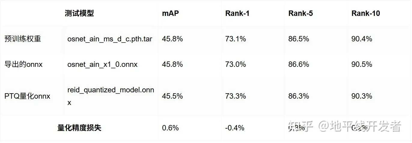
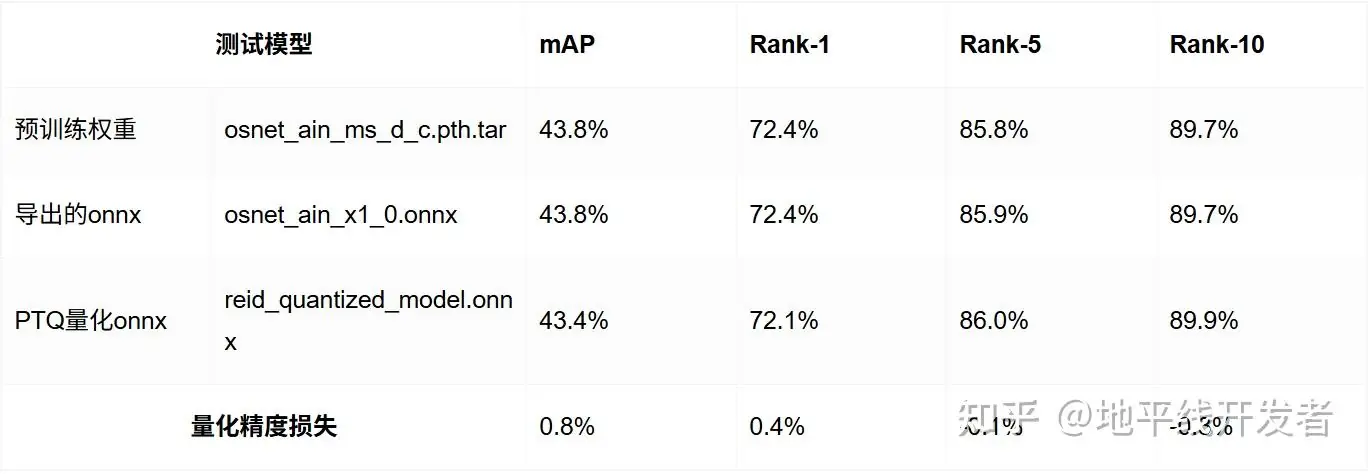
测试数据集：Market-1501-v15.09.15

1.距离度量方式：cosine

2.距离度量方式：euclidean

3.2 评测方法

3.2.1 预训练权重

在第一章配置好的官方运行环境中，使用代码仓库的现有方法对预训练权重做精度评测。

PYTHONPATH=. python3 scripts/main.py \
--config-file configs/im_osnet_ain_x1_0_softmax_256x128_amsgrad_cosine.yaml \
--root ./ \
model.load_weights ./osnet_ain_ms_d_c.pth.tar \
test.evaluate True

3.2.2 导出的 onnx

需要基于第一章配置好的官方运行环境，额外安装 onnxruntime 和 tqdm 模块。

pip install onnxruntime
pip install tqdm

测试时，datamanager 参数需要和 configs/im_osnet_ain_x1_0_softmax_256x128_amsgrad_cosine.yaml 对齐。

import cv2
import torch
import numpy as np
import onnxruntime as ort
from PIL import Image
from tqdm import tqdm

from torchreid.data import ImageDataManager
from torchreid.metrics import compute_distance_matrix, evaluate_rank

def extract_feature(img_path):
    img = cv2.imread(img_path)
    img = cv2.cvtColor(img, cv2.COLOR_BGR2RGB)
    img = Image.fromarray(img)
    img = transform(img)
    img = img.unsqueeze(0).numpy()
    feat = session.run(None, {input_name: img})[0]
    return feat[0]

def extract_features(dataset):
    features, pids, camids = [], [], []
    for img_path, pid, camid, _ in tqdm(dataset, desc="Extracting features"):
        feat = extract_feature(img_path)
        features.append(feat)
        pids.append(pid)
        camids.append(camid)
    return np.stack(features), np.array(pids), np.array(camids)

datamanager = ImageDataManager(
    use_gpu=False,
    root="./",
    sources=['market1501'],
    height=256,
    width=128,
    batch_size_train=64,
    batch_size_test=1,
    transforms=['random_flip', 'color_jitter']
)

if __name__ == "__main__":
    query_loader = datamanager.test_loader['market1501']['query']
    gallery_loader = datamanager.test_loader['market1501']['gallery']

    query = query_loader.dataset.query
    gallery = gallery_loader.dataset.gallery
    transform = query_loader.dataset.transform

    session = ort.InferenceSession('osnet_ain_x1_0.onnx', providers=['CPUExecutionProvider'])
    input_name = session.get_inputs()[0].name

    query_features, query_pids, query_camids = extract_features(query)
    gallery_features, gallery_pids, gallery_camids = extract_features(gallery)

    distmat = compute_distance_matrix(
        torch.tensor(query_features),
        torch.tensor(gallery_features),
        metric='cosine'
    ).numpy()

    cmc, mAP = evaluate_rank(
        distmat, query_pids, gallery_pids, query_camids, gallery_camids, use_cython=False
    )

    print("\n=== Market1501 Evaluation Results (ONNX model) ===")
    print(f"mAP     : {mAP:.2%}")
    print(f"Rank-1  : {cmc[0]:.2%}")
    print(f"Rank-5  : {cmc[4]:.2%}")
    print(f"Rank-10 : {cmc[9]:.2%}")

3.2.3 PTQ 量化 onnx

需要基于第一章配置好的官方运行环境，额外安装 onnxruntime 和 tqdm 模块，并安装 horizon-nn/hmct 和 horizon-tc-ui。

pip install onnxruntime
pip install tqdm
pip install horizon_nn-1.1.0.post0.dev202506060002+840a0a685d053923c1a577c5032b7e0cfc84e6ac-cp310-cp310-linux_x86_64.whl --no-deps
pip install horizon_tc_ui-1.24.4-cp310-cp310-linux_x86_64.whl --no-deps

测试时，datamanager 参数需要和 configs/im_osnet_ain_x1_0_softmax_256x128_amsgrad_cosine.yaml 对齐，且需要把输入数据处理成 yuv444 类型。

import cv2
import torch
import numpy as np
from PIL import Image
from tqdm import tqdm
from horizon_tc_ui import HB_ONNXRuntime

from torchreid.data import ImageDataManager
from torchreid.metrics import compute_distance_matrix, evaluate_rank

def bgr2nv12(image):
    image = image.astype(np.uint8) 
    height, width = image.shape[0], image.shape[1] 
    yuv420p = cv2.cvtColor(image, cv2.COLOR_BGR2YUV_I420).reshape((height * width * 3 // 2, )) 
    y = yuv420p[:height * width] 
    uv_planar = yuv420p[height * width:].reshape((2, height * width // 4)) 
    uv_packed = uv_planar.transpose((1, 0)).reshape((height * width // 2, )) 
    nv12 = np.zeros_like(yuv420p) 
    nv12[:height * width] = y 
    nv12[height * width:] = uv_packed 
    return nv12 
 
def nv12Toyuv444(nv12, target_size): 
    height = target_size[0] 
    width = target_size[1] 
    nv12_data = nv12.flatten() 
    yuv444 = np.empty([height, width, 3], dtype=np.uint8) 
    yuv444[:, :, 0] = nv12_data[:width * height].reshape(height, width) 
    u = nv12_data[width * height::2].reshape(height // 2, width // 2) 
    yuv444[:, :, 1] = Image.fromarray(u).resize((width, height),resample=0) 
    v = nv12_data[width * height + 1::2].reshape(height // 2, width // 2) 
    yuv444[:, :, 2] = Image.fromarray(v).resize((width, height),resample=0) 
    return yuv444 

def preprocess_nhwc(img_path):
    bgr_input = cv2.imread(img_path)
    bgr_input = cv2.resize(bgr_input, (128,256), interpolation=cv2.INTER_LINEAR)
    nv12_input = bgr2nv12(bgr_input)
    yuv444 = nv12Toyuv444(nv12_input, (256,128))
    yuv444 = yuv444[np.newaxis,:,:,:]
    return yuv444

def extract_feature(img_path):
    for input_name in input_names:
        feed_dict[input_name] = preprocess_nhwc(img_path)
    feat = sess.run(output_names, feed_dict)
    return feat[0]

def extract_features(dataset):
    features, pids, camids = [], [], []
    for img_path, pid, camid, _ in tqdm(dataset, desc="Extracting features"):
        feat = extract_feature(img_path)
        features.append(feat)
        pids.append(pid)
        camids.append(camid)
    return np.stack(features), np.array(pids), np.array(camids)

if __name__ == "__main__":
    datamanager = ImageDataManager(
        use_gpu=False,
        root="./",
        sources=['market1501'],
        height=256,
        width=128,
        batch_size_train=64,
        batch_size_test=1,
        transforms=['random_flip', 'color_jitter']
    )

    query_loader = datamanager.test_loader['market1501']['query']
    gallery_loader = datamanager.test_loader['market1501']['gallery']

    query = query_loader.dataset.query
    gallery = gallery_loader.dataset.gallery
    transform = query_loader.dataset.transform

    sess = HB_ONNXRuntime(model_file='./model_output_inx2_cpu/reid_quantized_model.onnx')
    input_names = [input.name for input in sess.get_inputs()]
    output_names = [output.name for output in sess.get_outputs()]
    feed_dict = dict()

    query_features, query_pids, query_camids = extract_features(query)
    gallery_features, gallery_pids, gallery_camids = extract_features(gallery)

    distmat = compute_distance_matrix(
        torch.tensor(query_features.squeeze(1)),
        torch.tensor(gallery_features.squeeze(1)),
        metric='cosine'
    ).numpy()

    cmc, mAP = evaluate_rank(
        distmat, query_pids, gallery_pids, query_camids, gallery_camids, use_cython=False
    )

    print("\n=== Market1501 Evaluation Results (ONNX model) ===")
    print(f"mAP     : {mAP:.2%}")
    print(f"Rank-1  : {cmc[0]:.2%}")
    print(f"Rank-5  : {cmc[4]:.2%}")
    print(f"Rank-10 : {cmc[9]:.2%}")

四、性能评测

4.1 评测结果

Running condition:
  Thread number is: 1
  Frame count   is: 1000
  Program run time: 51433.128000 ms
Perf result:
  Frame totally latency is: 51417.804688 ms
  Average    latency    is: 51.417805 ms
  Frame      rate       is: 19.442722 FPS

以 X5 为例，该模型的单线程推理延时为 51.4ms，对应 FPS 为 19.4

Latency 是指单流程推理模型所耗费的平均时间，重在表示在资源充足的情况下推理一帧的平均耗时，体现在上板运行是单核单线程统计。

FPS 是指多流程同时进行模型推理平均一秒推理的帧数，重在表示充分使用资源情况下模型的吞吐，体现在上板运行为单核多线程；统计方法是同时起多个线程进行模型推理，计算平均 1s 推理的总帧数。

Latency 与 FPS 的统计情景不同，Latency 为单流程（单核单线程）推理，FPS 为多流程（单核多线程）推理，因此推算不一致；若统计 FPS 时将流程（线程）数量设置为 1 ，则通过 Latency 推算 FPS 和测出的一致。

4.2 评测方法

可板端使用 hrt_model_exec 工具获取模型的实测性能数据，测试命令如下：

hrt_model_exec perf --model-file reid.bin --frame-count 1000 --thread-num 1