文章目录
摘要
本周对上周未完成的卷积神经网络进行实现,用于对手写数字的识别问题,准确率达到了70%,可能这与神经网络层数太少有关,学习卷积神经网络中的反向传播更新参数。同时也对多层感知机进行学习并进行代码实验。
Abstract
This week, the convolutional neural network that was not completed last week was implemented for the recognition of handwritten numbers, and the accuracy reached 70%, which may be related to the fact that the number of layers of the neural network is too small, and the backpropagation update parameters in the learning convolutional neural network are carried out. At the same time, the multi-layer perceptron is also learned and code experiments are conducted.
1卷积神经网络
书接上回,说到对卷积神经网络也进行了实验,但是实验的效果不好,准确率只有10%,十分的差,怀疑是自己的模型实现有问题。于是本周对这个实验重新做一次。
1.1卷积层
卷积神经网络先做卷积层。

图1.1 卷积操作
卷积操作类似上图,在绿色框框对图片进行卷积运算,直到运算完整个图片。例如:
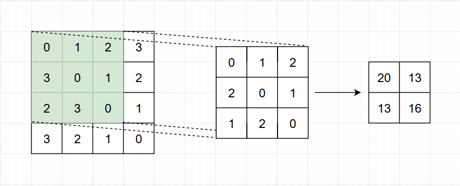
图1.2 卷积计算
卷积核对图像相同大小的区域(绿色部分)进行逐位相乘后相加
0 × 0 + 1 × 1 + 2 × 2 + 3 × 2 + 0 × 0 + 1 × 1 + 2 × 1 + 3 × 2 + 0 × 0 = 20 0\times 0+1\times 1 +2\times 2+3\times 2+0\times 0+1\times 1+2\times 1+3\times 2+0\times 0=20 0×0+1×1+2×2+3×2+0×0+1×1+2×1+3×2+0×0=20
以此类推。
先对一个图片进行卷积:
python
import pandas as pd
import numpy as np
import random
from sklearn.datasets import load_digits
import matplotlib.pyplot as plt
digits=load_digits()
data=digits.data[0].reshape((8,8))
plt.imshow(data,cmap=plt.cm.binary,interpolation='nearest')
def conv(data,kernel):
    height,width=data.shape
    output=np.zeros((height-2,width-2))
    for i in range(height-2):
        for j in range(width-2):
            window = data[i:i+3,j:j+3]
            output[i,j]=np.sum(kernel*window)
    return output
kernel = [[1,-1,-1],[-1,1,-1],[-1,-1,1]]
conv_data = conv(data,kernel)
plt.imshow(output,cmap=plt.cm.binary,interpolation='nearest')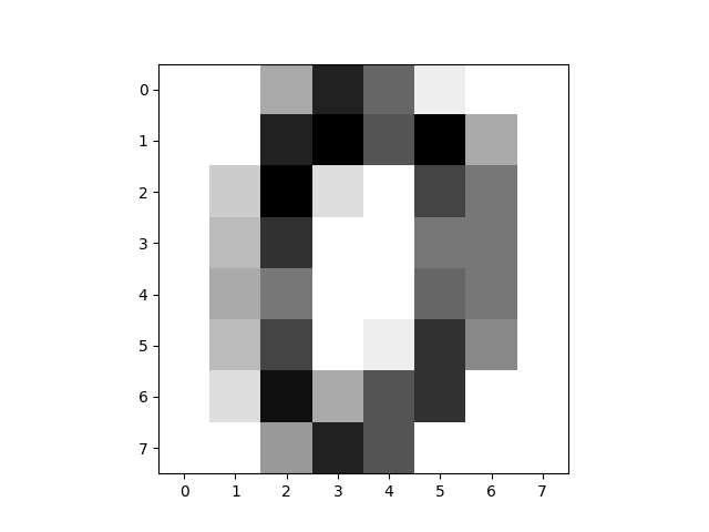
图1.3 卷积处理前
图1.4 卷积处理后
1.2 池化层
8 × 8 8\times 8 8×8维原始图像卷积后是 6 × 6 6\times 6 6×6维卷积处理会模糊图像,增强边缘。卷积处理完成后是池化处理,池化有最大池化、平均池化、全局平均池化、全局最大池化。
平均池化:计算图像区域的平均值作为该区域池化后的平均值。
最大池化:选图像区域的最大值作为该区域池化后的值。
平均池化会模糊关键特征,最大池化会突出选定区域的特征。在实验中,发现最大池化的效果好于平均池化。
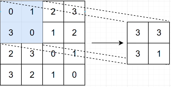
图1.5 最大池化
python
#池化层,data:卷积后的图片
def pool(data,window_size=2,stride=2):
    height, width = data.shape
    # 计算输出尺寸
    output_height = (height - window_size) // stride + 1
    output_width = (width - window_size) // stride + 1
    output = np.zeros((output_height, output_width))
    for i in range(0, height - window_size + 1, stride):
        for j in range(0, width - window_size + 1, stride):
            window = data[i:i+window_size, j:j+window_size]
            output[i//stride, j//stride] = np.max(window)
    return output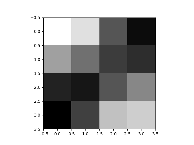
图1.6 平均池化后图像
1.3 全连接层
6 × 6 6\times 6 6×6维图像池化后是 3 × 3 3\times 3 3×3维,对图像展平成1维的向量。
python
def flatten(data):
    return data.reshape(-1)
展平后到全连接层,全连接层的输出 o u t p u t = i n p u t ∗ W + b output=input * W+b output=input∗W+b
展平后的图片向量是 1 × 9 1\times 9 1×9的向量,可以说是9个神经元,每个神经元都有一列特征值,然后全连接层有偏置b和权重矩阵w,权重矩阵w是9个神经元中,每个特征的权重。比如说展平数据的第一个值,是由权重矩阵第一列进行计算
o u t p u t 0 = w 00 f 0 + w 10 f 1 + w 20 f 2 + . . . + w 80 f 8 + b 0 output_0=w_{00}f_0+w_{10}f_1+w_{20}f_2+...+w_{80}f_8+b_0 output0=w00f0+w10f1+w20f2+...+w80f8+b0
o u t p u t 0 output_0 output0代表着是类别是0的概率,后续的训练就是在不断调整参数矩阵和偏置值。
最后通过输出np.argmax(output)得到最大的概率的类别作为预测类别。
以上是一次前向传播的过程。
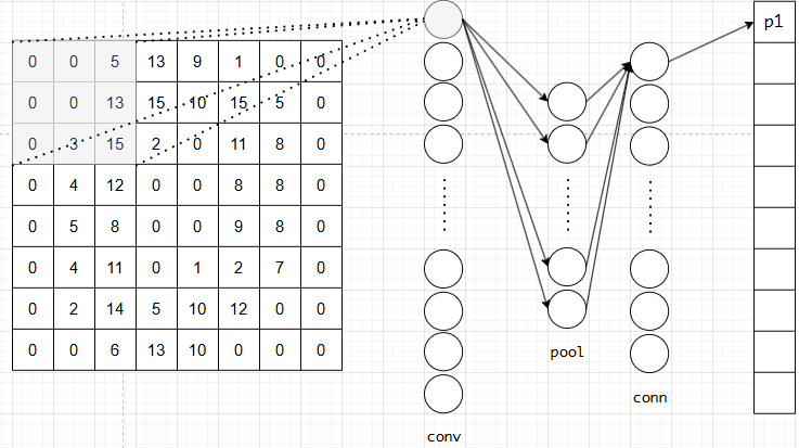
图1.7 神经网络
以上神经网络是实验中所做的卷积神经网络,卷积层有36个神经元,池化层有9个神经元,全连接层有10个神经元。
1.4 反向传播
对参数更新需要用到反向传播,反向传播前要先计算交叉熵 E E E
E = − ∑ i y ( i ) l o g P ( i ) E=- \sum_i y(i) log P(i) E=−∑iy(i)logP(i)
就是对每一个类别预测出来的概率乘以该类别的真实标签,对于多分类,将各个类进行独热编码。
比如把2编码成0,0,1,0,0,0,0,0,0,0,然后预测的概率为0.1,0.05,0.2,0.01,0.03,0.01,0.4,0.04,0.06,0.1
E = − 1 ∗ l o g 0.2 ≈ 0.6989 E=-1*log 0.2\approx0.6989 E=−1∗log0.2≈0.6989
交叉熵越小代表误差越小。
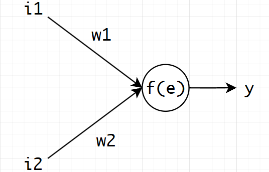
图 1.8神经元模型
y = i 1 × w 1 + i 2 × w 2 y=i1\times w1+i2 \times w2 y=i1×w1+i2×w2
卷积核也就是把输入变成9,权重变成9,所以卷积核也是参数,也需要进行更新。
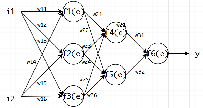
图1.9 神经网络模型
y 1 = f 1 ( i 1 w 11 + i 2 w 14 ) y 2 = f 2 ( i 1 w 12 + i 2 w 15 ) y 3 = f 3 ( i 1 w 13 + i 2 w 16 ) y 4 = f 4 ( y 1 w 21 + y 2 w 23 + y 3 w 25 ) y 5 = f 5 ( y 1 w 22 + y 2 w 24 + y 3 w 26 ) y = f 6 ( y 4 w 31 + y 5 w 32 ) \begin{aligned}y_1&=f_1(i_1 w_{11}+i_2 w_{14})\\ y_2&=f_2(i_1 w_{12}+i_2 w_{15}) \\ y_3&=f_3(i_1 w_{13}+i_2 w_{16}) \\ y_4&=f_4(y_1w_{21}+y_2w_{23}+y_3w_{25})\\ y_5&=f_5(y_1w_{22}+y_2w_{24}+y_3w_{26})\\ y&=f_6(y_4w_{31}+y_5w_{32})\end{aligned} y1y2y3y4y5y=f1(i1w11+i2w14)=f2(i1w12+i2w15)=f3(i1w13+i2w16)=f4(y1w21+y2w23+y3w25)=f5(y1w22+y2w24+y3w26)=f6(y4w31+y5w32)
反向转播
∂ L ∂ w 31 = ∂ L ∂ y ⋅ ∂ y ∂ f 6 ⋅ ∂ f 6 ∂ w 31 ∂ L ∂ w 32 = ∂ L ∂ y ⋅ ∂ y ∂ f 6 ⋅ ∂ f 6 ∂ w 32 ⋮ ∂ L ∂ w 11 = ∂ L ∂ y ⋅ ∂ y ∂ f 6 ( ∂ f 6 ∂ y 4 ⋅ ∂ y 4 ∂ f 4 ⋅ ∂ f 4 ∂ y 1 + ∂ f 6 ∂ y 5 ⋅ ∂ y 5 ∂ f 5 ⋅ ∂ f 5 ∂ y 1 ) ∂ y 1 ∂ f 1 ⋅ ∂ f 1 ∂ w 11 \begin{aligned} \frac{\partial L}{\partial w_{31}}&=\frac{\partial L}{\partial y}\cdot \frac{\partial y}{\partial f_6}\cdot \frac{\partial f_6}{\partial w_{31}} \\ \frac{\partial L}{\partial w_{32}}&=\frac{\partial L}{\partial y}\cdot \frac{\partial y}{\partial f_6}\cdot \frac{\partial f_6}{\partial w_{32}} \\ \vdots \\ \frac{\partial L}{\partial w_{11}}&=\frac{\partial L}{\partial y}\cdot \frac{\partial y}{\partial f_6}(\frac{\partial f_6}{\partial y_4}\cdot \frac{\partial y_4}{\partial f_4}\cdot \frac{\partial f_4}{\partial y_1} + \frac{\partial f_6}{\partial y_5}\cdot \frac{\partial y_5}{\partial f_5}\cdot \frac{\partial f_5}{\partial y_1}) \frac{\partial y_1}{\partial f_1}\cdot \frac{\partial f_1}{\partial w_{11}}\\ \end{aligned} ∂w31∂L∂w32∂L⋮∂w11∂L=∂y∂L⋅∂f6∂y⋅∂w31∂f6=∂y∂L⋅∂f6∂y⋅∂w32∂f6=∂y∂L⋅∂f6∂y(∂y4∂f6⋅∂f4∂y4⋅∂y1∂f4+∂y5∂f6⋅∂f5∂y5⋅∂y1∂f5)∂f1∂y1⋅∂w11∂f1
参数更新
w 11 = w 11 − l e a r n i n g _ r a t e × ∂ L ∂ w 11 w_{11}=w_{11}-learning\rate\times \frac{\partial L}{\partial w{11}} w11=w11−learning_rate×∂w11∂L
以此类推
1.5 CNN代码
python
import pandas as pd
import numpy as np
import random
from sklearn.datasets import load_digits
import matplotlib.pyplot as plt
from sklearn.model_selection import train_test_split
digits=load_digits()#1797,64

data=digits.data[:1500]
target=digits.target[:1500]
print(data[0])
x_train,x_test,y_train,y_test=train_test_split(data,target,
    test_size=0.2,
    random_state=2,
    shuffle=True)
def relu(x):
    return np.maximum(0, x)
def relu_derivative(x):
    return (x > 0).astype(np.float32)
#卷积层,data:原始图片,kernel:卷积核
def conv(data,kernel,window_size=3):
    data_height, data_width = data.shape
    kernel_height, kernel_width = kernel.shape

    # 计算输出尺寸
    output_height = data_height - kernel_height + 1
    output_width = data_width - kernel_width + 1

    # 初始化输出
    output = np.zeros((output_height, output_width))

    # 执行卷积
    for i in range(output_height):
        for j in range(output_width):
            window = data[i:i+kernel_height, j:j+kernel_width]
            output[i, j] = np.sum(kernel * window)

    return relu(output)
#池化层,data:卷积后的图片
def pool(data,window_size=2,stride=2):
    height, width = data.shape
    # 计算输出尺寸
    output_height = (height - window_size) // stride + 1
    output_width = (width - window_size) // stride + 1

    output = np.zeros((output_height, output_width))

    for i in range(0, height - window_size + 1, stride):
        for j in range(0, width - window_size + 1, stride):
            window = data[i:i+window_size, j:j+window_size]
            output[i//stride, j//stride] = np.max(window)
    return output
#展平层,data:池化后的数据
def flatten(data):
    return data.reshape(-1)
#全连接层,data:展平后的数据
def conn(data,w,b):
    output = np.dot(data,w)+b
    return output
#softmax函数,转化为概率
def softmax(data):
    ex = np.exp(data)
    return ex/np.sum(ex)
#独热编码
def one_hot_encode(label,num_classes=10):
    encoding=np.zeros(num_classes)
    encoding[label]=1
    return encoding
#计算交叉熵
def loss(data,one_hot_code):
    data = np.clip(data,1e-12,1.- 1e-12)
    return -np.sum(one_hot_code*np.log(data))
m = 9#flatten的维度
n = 10
w = np.random.randn(m, 10)
b = np.random.randn(10)

kernel = np.array([[1,-1,-1],[-1,1,-1],[-1,-1,1]],dtype=np.float32)

learning_rate = 0.01

def train(x_train, y_train, epochs=10):
    global w, b, kernel

    losses = []
    accuracies = []

    for epoch in range(epochs):
        epoch_loss = 0
        correct = 0
        total = 0

        for i in range(len(x_train)):
            # 获取当前样本
            x = x_train[i].reshape(8, 8)
            y = y_train[i]

            # 前向传播
            conv_data = conv(x, kernel)
            pool_data = pool(conv_data)

            flatten_data = flatten(pool_data)  # 展平输出
            conn_output = conn(flatten_data, w, b)  # 全连接层输出
            output = softmax(conn_output)  # 最终输出

            # 计算损失
            one_hot_code = one_hot_encode(y)
            l = loss(output, one_hot_code)
            epoch_loss += l

            # 计算准确率
            predicted = np.argmax(output)
            if predicted == y:
                correct += 1
            total += 1

            # 反向传播
            # 计算梯度
            dlz = output - one_hot_code  # 损失对全连接层输出的梯度

            # 计算全连接层参数的梯度
            dlw = np.outer(dlz, flatten_data)  # 损失对权重的梯度
            dlb = dlz  # 损失对偏置的梯度

            # 反向传播到池化层
            dl_pool = np.dot(w, dlz)  # 全连接层的反向传播
            dl_pool_reshaped = dl_pool.reshape(pool_data.shape)

            # 反向传播到卷积层
            # 平均池化的反向传播:将梯度均匀分配到每个输入元素
            dl_conv = np.zeros_like(conv_data, dtype=np.float32)
            pool_h, pool_w = pool_data.shape
            for i in range(pool_h):
                for j in range(pool_w):
                    window_grad = dl_pool_reshaped[i, j] / 9  # 3x3窗口,共9个元素
                    dl_conv[i:i+3, j:j+3] += window_grad

            # 应用ReLU的导数
            dl_conv = dl_conv * relu_derivative(conv_data)

            # 计算损失对卷积核的梯度
            dl_kernel = np.zeros_like(kernel, dtype=np.float32)
            conv_h, conv_w = conv_data.shape
            for i in range(conv_h):
                for j in range(conv_w):
                    window = x[i:i+3, j:j+3].astype(np.float32)
                    dl_kernel += window * dl_conv[i, j]

            # 更新参数
            w -= learning_rate * dlw.T
            b -= learning_rate * dlb
            kernel -= learning_rate * dl_kernel

        # 计算平均损失和准确率
        avg_loss = epoch_loss / len(x_train)
        accuracy = correct / total

        losses.append(avg_loss)
        accuracies.append(accuracy)

        if epoch % 5 == 0:
            print(f"Epoch {epoch+1}/{epochs}, Loss: {avg_loss:.4f}, Accuracy: {accuracy:.4f}")

    return losses, accuracies
# 测试函数
def test(x_test, y_test):
    correct = 0
    total = 0

    for i in range(len(x_test)):
        x = x_test[i].reshape(8, 8)
        y = y_test[i]

        # 前向传播
        conv_data = conv(x, kernel)
        pool_data = pool(conv_data)

        flatten_data = flatten(pool_data)
        conn_output = conn(flatten_data, w, b)
        output = softmax(conn_output)

        # 预测
        predicted = np.argmax(output)
        if predicted == y:
            correct += 1
        total += 1

    accuracy = correct / total
    print(f"测试准确率: {accuracy:.4f}")
    return accuracy
# 训练模型
print("开始训练...")
losses, accuracies = train(x_train, y_train, epochs=50)

# 测试模型
print("\n开始测试...")
test_accuracy = test(x_test, y_test)

# 绘制损失和准确率曲线
plt.figure(figsize=(12, 4))

plt.subplot(1, 2, 1)
plt.plot(losses)
plt.title('Training Loss')
plt.xlabel('Epoch')
plt.ylabel('Loss')

plt.subplot(1, 2, 2)
plt.plot(accuracies)
plt.title('Training Accuracy')
plt.xlabel('Epoch')
plt.ylabel('Accuracy')

plt.tight_layout()
plt.show()
'''
开始训练...
Epoch 1/50, Loss: 2.6471, Accuracy: 0.2525
Epoch 6/50, Loss: 1.6033, Accuracy: 0.3817
Epoch 11/50, Loss: 1.5698, Accuracy: 0.3933
Epoch 16/50, Loss: 1.5354, Accuracy: 0.4158
Epoch 21/50, Loss: 1.4275, Accuracy: 0.4675
Epoch 26/50, Loss: 1.3696, Accuracy: 0.5117
Epoch 31/50, Loss: 1.1931, Accuracy: 0.5700
Epoch 36/50, Loss: 1.3272, Accuracy: 0.6683
Epoch 41/50, Loss: 1.3060, Accuracy: 0.6675
Epoch 46/50, Loss: 0.9437, Accuracy: 0.7175

开始测试...
测试准确率: 0.7067
'''
这是单层神经网络经过50次训练的结果,后续会尝试堆叠多层。
使用的损失函数是交叉熵损失函数: E = − ∑ i y i l o g y i ^ E=-\sum_i y_ilog \hat{y_i} E=−∑iyilogyi^
输出层是softmax函数: f ( i ) = z i ∑ j e z j f(i)=\frac{z_i}{\sum_j e^{z_j}} f(i)=∑jezjzi
损失对输出的梯度: ∂ L ∂ z k = ∂ ( − ∑ i y i l o g y i ^ ) ∂ z k , z k ∈ s o f t m a x ( d a t a ) \frac{\partial L}{\partial z_k}=\frac{\partial (-\sum_i y_ilog\hat{y_i})}{\partial z_k},z_k\in softmax(data) ∂zk∂L=∂zk∂(−∑iyilogyi^),zk∈softmax(data), z k z_k zk是预测值的第k个值
i i i是常数,所以 ∂ L ∂ z k = ∂ ( − ∑ i y i l o g y i ^ ) ∂ z k = − ∑ i y i ∂ l o g y i ^ ∂ z k \frac{\partial L}{\partial z_k}=\frac{\partial (-\sum_i y_ilog\hat{y_i})}{\partial z_k}=-\sum_i y_i\frac{\partial log \hat{y_i}}{\partial z_k} ∂zk∂L=∂zk∂(−∑iyilogyi^)=−∑iyi∂zk∂logyi^
∂ l o g y i ^ ∂ z k = 1 y i ^ ∂ y i ^ ∂ z k \frac{\partial log\hat{y_i}}{\partial z_k}=\frac{1}{\hat{y_i}}\frac{\partial \hat{y_i}}{\partial z_k} ∂zk∂logyi^=yi^1∂zk∂yi^
∂ L ∂ z k = − ∑ i y i 1 y i ^ ∂ y i ^ ∂ z k \frac{\partial L}{\partial z_k}=-\sum_i y_i\frac{1}{\hat{y_i}}\frac{\partial \hat{y_i}}{\partial z_k} ∂zk∂L=−∑iyiyi^1∂zk∂yi^
要计算 ∂ y ^ ( i ) ∂ z k \frac{\partial \hat{y}(i)}{\partial z_k} ∂zk∂y^(i)取决于
(1) i = k i=k i=k, ∂ y i ^ ∂ z k = y i ^ ( 1 − y i ^ ) \frac{\partial \hat{y_i}}{\partial z_k}=\hat{y_i}(1-\hat{y_i}) ∂zk∂yi^=yi^(1−yi^)
(2) i ≠ k i\neq k i=k, ∂ y i ^ ∂ z k = − y i ^ y k ^ \frac{\partial \hat{y_i}}{\partial z_k}=-\hat{y_i}\hat{y_k} ∂zk∂yi^=−yi^yk^
最后 ∂ L ∂ z k = − ( y k − y k ^ ∑ i y i ) \frac{\partial L}{\partial z_k}=-(y_k-\hat{y_k}\sum_i y_i) ∂zk∂L=−(yk−yk^∑iyi)
经过独热编码后 ∑ i y i \sum_i y_i ∑iyi等于1
所以 ∂ L ∂ z k = y k ^ − y k \frac{\partial L}{\partial z_k}=\hat{y_k}-y_k ∂zk∂L=yk^−yk
接下来计算误差对参数的梯度 ∂ L ∂ w \frac{\partial L}{\partial w} ∂w∂L
∵ z = w T ∗ x + b ∂ L ∂ w = ∂ L ∂ z ⋅ ∂ z ∂ w ∵ ∂ L ∂ z k = y k ^ − y k ∂ L ∂ w = ( y k ^ − y k ) x \begin{aligned}\because z&=w^T*x+b \\ \frac{\partial L}{\partial w}&=\frac{\partial L}{\partial z}\cdot \frac{\partial z}{\partial w} \\ \because \frac{\partial L}{\partial z_k}&=\hat{y_k}-y_k \\ \frac{\partial L}{\partial w}&=(\hat{y_k}-y_k)x\end{aligned} ∵z∂w∂L∵∂zk∂L∂w∂L=wT∗x+b=∂z∂L⋅∂w∂z=yk^−yk=(yk^−yk)x
2 MLP
上周学习了单层感知机,这周学习多层感知机,多层感知机也叫人工神经网络(ANN),中间包含多个隐藏层,从易于理解起见,先学习三层感知机。
2.1 感知机模型
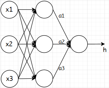
图2.1 多层感知机
多层感知机之间是全连接的。隐藏层与隐藏层之间通过函数 f ( w x + b ) f(wx+b) f(wx+b)进行连接。 f f f可以是sigmoid函数或者tanh函数。
σ ( x ) = 1 1 + e − x \sigma(x)=\frac{1}{1+e^{-x}} σ(x)=1+e−x1,导数为 σ ′ ( x ) = σ ( x ) ( 1 − σ ( x ) ) \sigma^{'}(x)=\sigma(x)(1-\sigma(x)) σ′(x)=σ(x)(1−σ(x))
反向传播:计算损失对参数的梯度,MLP一般使用均方误差函数: E = 1 m ∑ i = 1 m 1 k ∑ j = 1 k ( y i j ^ − y i j ) 2 E=\frac{1}{m}\sum_{i=1}^m\frac{1}{k}\sum_{j=1}^k(\hat{y_{ij}}-y_{ij})^2 E=m1∑i=1mk1∑j=1k(yij^−yij)2
m为训练样本个数,k为输出个数, y i j ^ \hat{y_{ij}} yij^为第i个样本第j个输出的预测值, y i j y_{ij} yij为对应的真实值
2.2 代码实现
python
import numpy as np
import matplotlib.pyplot as plt
from sklearn.datasets import load_digits
from sklearn.model_selection import train_test_split
from sklearn.preprocessing import StandardScaler

# 加载数据
digits = load_digits()
data = digits.data
target = digits.target

# 数据预处理
scaler = StandardScaler()
data = scaler.fit_transform(data)

# 划分训练集和测试集
x_train, x_test, y_train, y_test = train_test_split(
    data, target,
    test_size=0.2,
    random_state=42,
    shuffle=True
)

# 激活函数
def relu(x):
    return np.maximum(0, x)

def relu_derivative(x):
    return (x > 0).astype(float)

def softmax(x):
    # 数值稳定的softmax
    exp_x = np.exp(x - np.max(x, axis=1, keepdims=True))
    return exp_x / np.sum(exp_x, axis=1, keepdims=True)

# MLP类
class MLP:
    def __init__(self, input_size, hidden_size, output_size):
        # He初始化权重
        self.w1 = np.random.randn(input_size, hidden_size) * np.sqrt(2. / input_size)
        self.b1 = np.zeros(hidden_size)
        self.w2 = np.random.randn(hidden_size, output_size) * np.sqrt(2. / hidden_size)
        self.b2 = np.zeros(output_size)

    def forward(self, X):
        # 隐藏层
        self.z1 = np.dot(X, self.w1) + self.b1
        self.a1 = relu(self.z1)

        # 输出层
        self.z2 = np.dot(self.a1, self.w2) + self.b2
        self.a2 = softmax(self.z2)

        return self.a2

    def backward(self, X, y, output, lr):
        # 样本数量
        m = X.shape[0]

        # 输出层梯度
        dz2 = (output - y) / m

        # 隐藏层梯度
        dz1 = np.dot(dz2, self.w2.T) * relu_derivative(self.z1)

        # 计算梯度
        dw2 = np.dot(self.a1.T, dz2)
        db2 = np.sum(dz2, axis=0)
        dw1 = np.dot(X.T, dz1)
        db1 = np.sum(dz1, axis=0)

        # 更新参数
        self.w1 -= lr * dw1
        self.b1 -= lr * db1
        self.w2 -= lr * dw2
        self.b2 -= lr * db2

    def train(self, X, y, epochs=100, lr=0.01, batch_size=32):
        losses = []
        accuracies = []

        # 将标签转换为one-hot编码
        y_onehot = np.zeros((len(y), 10))
        y_onehot[np.arange(len(y)), y] = 1

        for epoch in range(epochs):
            epoch_loss = 0
            correct = 0

            # 小批量训练
            for i in range(0, len(X), batch_size):
                # 获取当前批次
                X_batch = X[i:i+batch_size]
                y_batch = y_onehot[i:i+batch_size]

                # 前向传播
                output = self.forward(X_batch)

                # 计算损失
                loss = -np.sum(y_batch * np.log(output + 1e-8)) / len(X_batch)
                epoch_loss += loss * len(X_batch)

                # 计算准确率
                predictions = np.argmax(output, axis=1)
                true_labels = np.argmax(y_batch, axis=1)
                correct += np.sum(predictions == true_labels)

                # 反向传播
                self.backward(X_batch, y_batch, output, lr)

            # 计算平均损失和准确率
            avg_loss = epoch_loss / len(X)
            accuracy = correct / len(X)
            losses.append(avg_loss)
            accuracies.append(accuracy)

            if epoch % 10 == 0:
                print(f"Epoch {epoch}/{epochs}, Loss: {avg_loss:.4f}, Accuracy: {accuracy:.4f}")

        return losses, accuracies

    def predict(self, X):
        output = self.forward(X)
        return np.argmax(output, axis=1)

    def evaluate(self, X, y):
        predictions = self.predict(X)
        accuracy = np.mean(predictions == y)
        return accuracy

# 创建模型
input_size = x_train.shape[1]
hidden_size = 128  # 增加隐藏层大小
output_size = 10

mlp = MLP(input_size, hidden_size, output_size)

# 训练模型
print("开始训练...")
losses, accuracies = mlp.train(x_train, y_train, epochs=100, lr=0.01, batch_size=64)

# 测试模型
print("\n开始测试...")
test_accuracy = mlp.evaluate(x_test, y_test)
print(f"测试准确率: {test_accuracy:.4f}")

# 绘制结果
plt.figure(figsize=(12, 5))

plt.subplot(1, 2, 1)
plt.plot(losses)
plt.title('Training Loss')
plt.xlabel('Epoch')
plt.ylabel('Loss')

plt.subplot(1, 2, 2)
plt.plot(accuracies)
plt.title('Training Accuracy')
plt.xlabel('Epoch')
plt.ylabel('Accuracy')

plt.tight_layout()
plt.show()
'''
开始训练...
Epoch 0/100, Loss: 2.7099, Accuracy: 0.1538
Epoch 10/100, Loss: 0.5566, Accuracy: 0.8727
Epoch 20/100, Loss: 0.3300, Accuracy: 0.9297
Epoch 30/100, Loss: 0.2409, Accuracy: 0.9506
Epoch 40/100, Loss: 0.1910, Accuracy: 0.9624
Epoch 50/100, Loss: 0.1582, Accuracy: 0.9708
Epoch 60/100, Loss: 0.1348, Accuracy: 0.9770
Epoch 70/100, Loss: 0.1171, Accuracy: 0.9805
Epoch 80/100, Loss: 0.1032, Accuracy: 0.9833
Epoch 90/100, Loss: 0.0920, Accuracy: 0.9854

开始测试...
测试准确率: 0.9583
'''
总结
本周学习了卷积神经网络和多层感知机并做了代码上的实现,对卷积神经网络中的反向传播仍有一点点不理解的部分,下周将会继续学习卷积神经网络的反向传播、多层感知机的反向传播以及RNN。