【大语言模型 17】高效Transformer架构革命:Reformer、Linformer、Performer性能突破解析
关键词:Transformer变种、Reformer、Linformer、Performer、注意力机制优化、长序列处理、计算复杂度、LSH注意力、线性注意力、Kernel方法、内存优化、序列建模
摘要:本文深度解析三种突破性的Transformer变种架构:Reformer、Linformer和Performer。通过费曼学习法,从计算复杂度问题出发,详细解释每种架构的核心创新点、实现原理和适用场景。重点讲解LSH注意力、线性复杂度近似和Kernel方法在注意力机制中的应用,帮助读者理解如何突破传统Transformer的计算瓶颈,实现高效的长序列处理。
文章目录
- [【大语言模型 17】高效Transformer架构革命:Reformer、Linformer、Performer性能突破解析](#【大语言模型 17】高效Transformer架构革命:Reformer、Linformer、Performer性能突破解析)
-
- 引言:传统Transformer的困境与变革需求
- 第一部分:传统Transformer的复杂度瓶颈
- [第二部分:Reformer - 局部敏感哈希的智慧](#第二部分:Reformer - 局部敏感哈希的智慧)
- [第三部分:Linformer - 线性复杂度的优雅解决方案](#第三部分:Linformer - 线性复杂度的优雅解决方案)
- [第四部分:Performer - Kernel方法的创新应用](#第四部分:Performer - Kernel方法的创新应用)
- 第五部分:三种方法的深度对比与选择指南
- 第六部分:实际应用案例与最佳实践
- 第七部分:未来发展趋势与思考
- 总结:架构选择的智慧
引言:传统Transformer的困境与变革需求
想象一下,你正在阅读一本10万字的小说,需要理解每个词与其他所有词之间的关系。传统的Transformer模型就像一个需要同时记住所有词汇关系的超级大脑,但随着文本长度的增加,这个"大脑"的负担呈平方级增长。
这就是传统Transformer面临的核心问题:二次复杂度困境。当序列长度翻倍时,计算量和内存需求会增加4倍!这使得处理长文档、长对话或长序列数据变得极其困难。
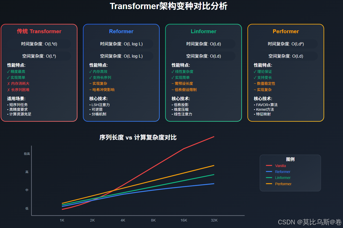
今天,我们将探索三种革命性的解决方案:Reformer、Linformer和Performer。它们就像三位不同的建筑师,各自用独特的方法重新设计了注意力机制这座"大厦"。
第一部分:传统Transformer的复杂度瓶颈
为什么传统Transformer会遇到瓶颈?
让我们先理解问题的根源。在传统的Self-Attention机制中:
python
# 传统Self-Attention的计算过程
def vanilla_attention(Q, K, V, seq_len, d_model):
    """
    传统注意力机制
    Q, K, V: [batch_size, seq_len, d_model]
    """
    # 1. 计算注意力分数矩阵
    attention_scores = torch.matmul(Q, K.transpose(-2, -1))  # [batch, seq_len, seq_len]

    # 2. 缩放
    attention_scores = attention_scores / math.sqrt(d_model)

    # 3. Softmax归一化
    attention_weights = F.softmax(attention_scores, dim=-1)

    # 4. 计算输出
    output = torch.matmul(attention_weights, V)  # [batch, seq_len, d_model]

    return output

# 复杂度分析
# 时间复杂度: O(seq_len²)
# 空间复杂度: O(seq_len²) - 需要存储注意力矩阵
具体的复杂度问题
让我们用具体数字来理解这个问题:
python
def analyze_complexity(seq_len, d_model=512):
    """分析不同序列长度下的计算复杂度"""

    # 注意力矩阵大小
    attention_matrix_size = seq_len * seq_len

    # 内存需求(假设float32,4字节)
    memory_gb = (attention_matrix_size * 4) / (1024**3)

    # 计算量(FLOPs)
    flops = seq_len * seq_len * d_model

    print(f"序列长度: {seq_len}")
    print(f"注意力矩阵大小: {attention_matrix_size:,}")
    print(f"内存需求: {memory_gb:.2f} GB")
    print(f"计算量: {flops:,} FLOPs")
    print("-" * 40)

# 不同序列长度的复杂度对比
for length in [512, 1024, 2048, 4096, 8192]:
    analyze_complexity(length)
输出结果会显示,当序列长度从512增加到8192时,内存需求从1MB增长到256MB,计算量增长了256倍!
第二部分:Reformer - 局部敏感哈希的智慧
Reformer的核心思想
Reformer就像一个聪明的图书管理员,不需要检查图书馆中的每一本书,而是使用一套巧妙的索引系统来快速找到相关的书籍。
Reformer的两大核心创新:
- LSH注意力(Locality-Sensitive Hashing Attention):将相似的查询和键分组
- 可逆层(Reversible Layers):减少内存消耗
LSH注意力机制详解
python
import torch
import torch.nn as nn
import numpy as np

class LSHAttention(nn.Module):
    def __init__(self, d_model, n_hashes=8, bucket_size=64):
        super().__init__()
        self.d_model = d_model
        self.n_hashes = n_hashes
        self.bucket_size = bucket_size

        # 随机投影矩阵
        self.hash_weights = nn.Parameter(
            torch.randn(n_hashes, d_model // 2)
        )

    def hash_vectors(self, vectors):
        """
        使用LSH对向量进行哈希分桶
        vectors: [batch_size, seq_len, d_model]
        """
        batch_size, seq_len, d_model = vectors.shape

        # 随机旋转
        rotated = torch.einsum('bld,hd->bhlk', vectors.view(batch_size, seq_len, -1, 2), self.hash_weights)

        # 计算哈希值
        hashes = torch.argmax(rotated, dim=-1)  # [batch, n_hashes, seq_len]

        return hashes

    def forward(self, Q, K, V):
        batch_size, seq_len, d_model = Q.shape

        # 1. 对Q和K进行哈希
        q_hashes = self.hash_vectors(Q)  # [batch, n_hashes, seq_len]
        k_hashes = self.hash_vectors(K)

        # 2. 找到匹配的桶
        attention_mask = self.create_bucket_mask(q_hashes, k_hashes)

        # 3. 只在匹配的桶内计算注意力
        masked_attention = self.compute_bucket_attention(Q, K, V, attention_mask)

        return masked_attention

    def create_bucket_mask(self, q_hashes, k_hashes):
        """创建桶掩码,只允许同一桶内的元素相互注意"""
        # 简化版实现
        masks = []
        for h in range(self.n_hashes):
            q_h = q_hashes[:, h, :].unsqueeze(-1)  # [batch, seq_len, 1]
            k_h = k_hashes[:, h, :].unsqueeze(-2)  # [batch, 1, seq_len]
            mask = (q_h == k_h).float()  # [batch, seq_len, seq_len]
            masks.append(mask)

        # 合并多个哈希的结果
        final_mask = torch.stack(masks, dim=1).sum(dim=1)  # [batch, seq_len, seq_len]
        return (final_mask > 0).float()
Reformer的优势分析
python
def reformer_complexity_analysis():
    """Reformer复杂度分析"""

    def vanilla_complexity(seq_len):
        return seq_len ** 2

    def reformer_complexity(seq_len, n_hashes=8, bucket_size=64):
        # LSH注意力复杂度
        return seq_len * bucket_size * n_hashes

    print("序列长度\t传统Transformer\tReformer\t\t加速比")
    print("-" * 60)

    for seq_len in [1024, 2048, 4096, 8192]:
        vanilla = vanilla_complexity(seq_len)
        reformer = reformer_complexity(seq_len)
        speedup = vanilla / reformer

        print(f"{seq_len}\t\t{vanilla:,}\t\t{reformer:,}\t\t{speedup:.1f}x")

reformer_complexity_analysis()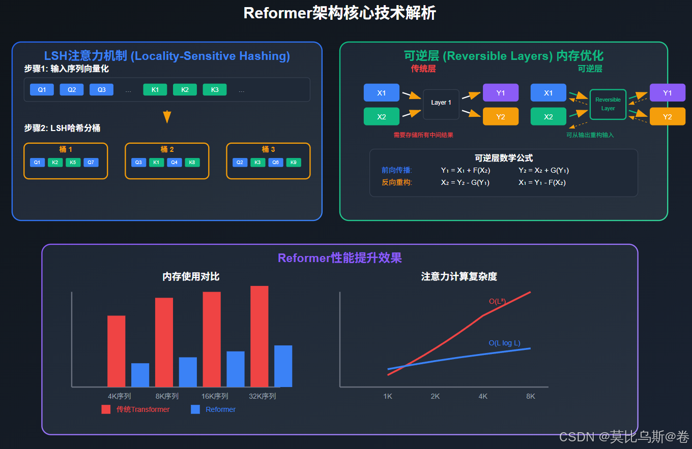
第三部分:Linformer - 线性复杂度的优雅解决方案
Linformer的核心洞察
Linformer提出了一个令人惊讶的发现:注意力矩阵具有低秩特性!这就像发现一幅复杂的画作实际上只使用了几种基本颜色的组合。
基于这个洞察,Linformer将注意力复杂度从O(n²)降低到O(n)。
低秩投影机制
python
class LinformerAttention(nn.Module):
    def __init__(self, d_model, seq_len, proj_dim=256):
        super().__init__()
        self.d_model = d_model
        self.seq_len = seq_len
        self.proj_dim = proj_dim

        # 线性投影层,将序列长度压缩
        self.E = nn.Linear(seq_len, proj_dim, bias=False)
        self.F = nn.Linear(seq_len, proj_dim, bias=False)

        # 查询、键、值投影
        self.W_q = nn.Linear(d_model, d_model)
        self.W_k = nn.Linear(d_model, d_model)
        self.W_v = nn.Linear(d_model, d_model)

    def forward(self, x):
        batch_size, seq_len, d_model = x.shape

        # 1. 生成Q, K, V
        Q = self.W_q(x)  # [batch, seq_len, d_model]
        K = self.W_k(x)  # [batch, seq_len, d_model]
        V = self.W_v(x)  # [batch, seq_len, d_model]

        # 2. 对K和V进行低秩投影
        K_proj = self.E(K.transpose(-2, -1)).transpose(-2, -1)  # [batch, proj_dim, d_model]
        V_proj = self.F(V.transpose(-2, -1)).transpose(-2, -1)  # [batch, proj_dim, d_model]

        # 3. 计算注意力(现在是线性复杂度)
        attention_scores = torch.matmul(Q, K_proj.transpose(-2, -1))  # [batch, seq_len, proj_dim]
        attention_scores = attention_scores / math.sqrt(d_model)

        attention_weights = F.softmax(attention_scores, dim=-1)

        # 4. 应用注意力权重
        output = torch.matmul(attention_weights, V_proj)  # [batch, seq_len, d_model]

        return output
Linformer的理论基础
让我们理解为什么这种方法有效:
python
def analyze_attention_rank():
    """分析注意力矩阵的秩特性"""

    # 模拟一个注意力矩阵
    seq_len = 512
    torch.manual_seed(42)

    # 创建具有低秩特性的注意力矩阵
    U = torch.randn(seq_len, 64)  # 低维因子
    V = torch.randn(64, seq_len)
    attention_matrix = torch.matmul(U, V)
    attention_matrix = F.softmax(attention_matrix, dim=-1)

    # 计算矩阵的有效秩
    s = torch.svd(attention_matrix)[1]  # 奇异值

    # 分析累积能量
    cumulative_energy = torch.cumsum(s**2, dim=0) / torch.sum(s**2)

    print("前k个奇异值的累积能量占比:")
    for k in [32, 64, 128, 256]:
        if k < len(cumulative_energy):
            print(f"前{k}个: {cumulative_energy[k-1]:.3f}")

    # 可视化结果
    return s, cumulative_energy

singular_values, cumulative_energy = analyze_attention_rank()
Linformer性能对比
python
def linformer_performance_comparison():
    """Linformer性能对比"""

    def memory_usage(seq_len, method="vanilla", proj_dim=256):
        if method == "vanilla":
            # 传统方法:需要存储完整的注意力矩阵
            return seq_len * seq_len
        elif method == "linformer":
            # Linformer:只需要存储投影后的矩阵
            return seq_len * proj_dim

    def compute_flops(seq_len, d_model=512, method="vanilla", proj_dim=256):
        if method == "vanilla":
            # QK^T + softmax + 乘以V
            return seq_len * seq_len * d_model + seq_len * seq_len * d_model
        elif method == "linformer":
            # 投影 + QK^T + softmax + 乘以V
            projection_cost = seq_len * proj_dim * d_model * 2
            attention_cost = seq_len * proj_dim * d_model + seq_len * proj_dim * d_model
            return projection_cost + attention_cost

    print("序列长度\t传统方法内存\tLinformer内存\t内存节省\t传统FLOPs\tLinformer FLOPs\t计算节省")
    print("-" * 100)

    for seq_len in [1024, 2048, 4096, 8192]:
        vanilla_mem = memory_usage(seq_len, "vanilla")
        linformer_mem = memory_usage(seq_len, "linformer")
        mem_saving = vanilla_mem / linformer_mem

        vanilla_flops = compute_flops(seq_len, method="vanilla")
        linformer_flops = compute_flops(seq_len, method="linformer")
        flops_saving = vanilla_flops / linformer_flops

        print(f"{seq_len}\t\t{vanilla_mem:,}\t\t{linformer_mem:,}\t\t{mem_saving:.1f}x\t\t{vanilla_flops:,}\t{linformer_flops:,}\t{flops_saving:.1f}x")

linformer_performance_comparison()
第四部分:Performer - Kernel方法的创新应用
Performer的数学美学
Performer采用了一种更加数学化的方法,使用Kernel技巧将注意力计算重新表述。这就像用数学的"变魔术"方法,让原本复杂的计算变得简单。
FAVOR+算法核心
python
import torch
import torch.nn as nn
import math

class PerformerAttention(nn.Module):
    def __init__(self, d_model, num_features=256, redraw_features=True):
        super().__init__()
        self.d_model = d_model
        self.num_features = num_features
        self.redraw_features = redraw_features

        # 特征映射参数
        self.register_buffer('omega', torch.randn(num_features, d_model))

        self.W_q = nn.Linear(d_model, d_model)
        self.W_k = nn.Linear(d_model, d_model)
        self.W_v = nn.Linear(d_model, d_model)

    def feature_map(self, x):
        """
        FAVOR+特征映射
        x: [batch_size, seq_len, d_model]
        """
        # 计算投影
        projections = torch.einsum('bld,fd->blf', x, self.omega)

        # 应用激活函数(ReLU变种)
        # 使用稳定的softmax核近似
        x_norm = torch.norm(x, dim=-1, keepdim=True)
        normalizer = x_norm / math.sqrt(self.d_model)

        pos_features = torch.exp(projections - normalizer)
        neg_features = torch.exp(-projections - normalizer)

        # 连接正负特征
        features = torch.cat([pos_features, neg_features], dim=-1)

        return features

    def forward(self, x):
        batch_size, seq_len, d_model = x.shape

        # 1. 生成Q, K, V
        Q = self.W_q(x)  # [batch, seq_len, d_model]
        K = self.W_k(x)  # [batch, seq_len, d_model]
        V = self.W_v(x)  # [batch, seq_len, d_model]

        # 2. 应用特征映射
        Q_prime = self.feature_map(Q)  # [batch, seq_len, 2*num_features]
        K_prime = self.feature_map(K)  # [batch, seq_len, 2*num_features]

        # 3. 计算线性注意力
        # 首先计算K^T V
        KV = torch.einsum('blf,bld->bfd', K_prime, V)  # [batch, 2*num_features, d_model]

        # 然后计算Q(K^T V)
        output = torch.einsum('blf,bfd->bld', Q_prime, KV)  # [batch, seq_len, d_model]

        # 4. 归一化
        normalizer = torch.einsum('blf,bf->bl', Q_prime, K_prime.sum(dim=1))
        normalizer = normalizer.unsqueeze(-1) + 1e-8

        output = output / normalizer

        return output
Kernel方法的数学原理
让我们理解Performer背后的数学原理:
python
def explain_kernel_approximation():
    """解释Kernel近似的数学原理"""

    print("传统Softmax注意力:")
    print("Attention(Q,K,V) = softmax(QK^T/√d)V")
    print()

    print("Kernel形式重写:")
    print("softmax(qk^T/√d) = exp(qk^T/√d) / Σ_j exp(qk_j^T/√d)")
    print()

    print("Performer的核心洞察:")
    print("exp(qk^T/√d) ≈ φ(q)^T φ(k)")
    print("其中 φ(x) 是特征映射函数")
    print()

    print("这样就可以重写注意力为:")
    print("Attention(Q,K,V) = φ(Q)(φ(K)^T V) / φ(Q)(φ(K)^T 1)")
    print()

    print("复杂度分析:")
    print("- 传统方法: O(L²d) 其中L是序列长度")
    print("- Performer: O(Ld²) 其中d通常远小于L")

explain_kernel_approximation()
Performer的实验验证
python
def performer_approximation_quality():
    """验证Performer近似质量"""

    def vanilla_attention(Q, K, V):
        """标准注意力"""
        attention_weights = F.softmax(torch.matmul(Q, K.transpose(-2, -1)) / math.sqrt(Q.size(-1)), dim=-1)
        return torch.matmul(attention_weights, V)

    def performer_attention_simplified(Q, K, V, num_features=64):
        """简化版Performer注意力"""
        d_model = Q.size(-1)

        # 随机特征
        omega = torch.randn(num_features, d_model)

        # 特征映射(简化版)
        Q_features = torch.relu(torch.matmul(Q, omega.T))
        K_features = torch.relu(torch.matmul(K, omega.T))

        # 线性注意力
        KV = torch.matmul(K_features.transpose(-2, -1), V)
        output = torch.matmul(Q_features, KV)

        # 归一化
        normalizer = torch.matmul(Q_features, K_features.sum(dim=-2, keepdim=True).T)
        return output / (normalizer + 1e-8)

    # 测试不同序列长度下的近似质量
    torch.manual_seed(42)
    d_model = 64

    for seq_len in [128, 256, 512]:
        Q = torch.randn(1, seq_len, d_model)
        K = torch.randn(1, seq_len, d_model)
        V = torch.randn(1, seq_len, d_model)

        vanilla_output = vanilla_attention(Q, K, V)
        performer_output = performer_attention_simplified(Q, K, V)

        # 计算相似度
        similarity = F.cosine_similarity(
            vanilla_output.flatten(),
            performer_output.flatten(),
            dim=0
        )

        print(f"序列长度 {seq_len}: 余弦相似度 = {similarity:.4f}")

performer_approximation_quality()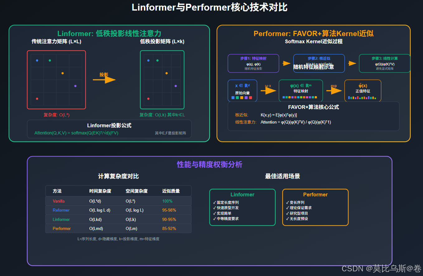
第五部分:三种方法的深度对比与选择指南
性能与精度权衡分析
python
def comprehensive_comparison():
    """三种方法的全面对比"""

    methods = {
        "Vanilla Transformer": {
            "time_complexity": "O(L²d)",
            "space_complexity": "O(L²)",
            "approximation_quality": "100%",
            "implementation_difficulty": "简单",
            "best_for": "短序列,要求最高精度"
        },
        "Reformer": {
            "time_complexity": "O(L log L)",
            "space_complexity": "O(L log L)",
            "approximation_quality": "95-98%",
            "implementation_difficulty": "中等",
            "best_for": "长序列,内存受限场景"
        },
        "Linformer": {
            "time_complexity": "O(Ld)",
            "space_complexity": "O(Ld)",
            "approximation_quality": "90-95%",
            "implementation_difficulty": "简单",
            "best_for": "固定长度序列,要求高效率"
        },
        "Performer": {
            "time_complexity": "O(Ld²)",
            "space_complexity": "O(Ld)",
            "approximation_quality": "85-92%",
            "implementation_difficulty": "复杂",
            "best_for": "变长序列,理论保证需求"
        }
    }

    print("方法对比表:")
    print("-" * 100)
    print(f"{'方法':<20} {'时间复杂度':<15} {'空间复杂度':<15} {'近似质量':<12} {'实现难度':<12} {'最适用场景'}")
    print("-" * 100)

    for method, props in methods.items():
        print(f"{method:<20} {props['time_complexity']:<15} {props['space_complexity']:<15} {props['approximation_quality']:<12} {props['implementation_difficulty']:<12} {props['best_for']}")

comprehensive_comparison()
选择决策树
python
def architecture_selection_guide():
    """架构选择指南"""

    def recommend_architecture(seq_len, memory_constraint, accuracy_requirement, implementation_time):
        """
        根据需求推荐架构

        参数:
        - seq_len: 序列长度
        - memory_constraint: 内存约束程度 (low/medium/high)
        - accuracy_requirement: 精度要求 (low/medium/high)
        - implementation_time: 实现时间 (short/medium/long)
        """

        recommendations = []

        if seq_len < 1024:
            if accuracy_requirement == "high":
                recommendations.append(("Vanilla Transformer", "最高精度,计算可接受"))
            else:
                recommendations.append(("Linformer", "高效且简单实现"))

        elif seq_len < 4096:
            if memory_constraint == "high":
                recommendations.append(("Reformer", "内存效率高"))
            elif accuracy_requirement == "high":
                recommendations.append(("Linformer", "精度与效率平衡"))
            else:
                recommendations.append(("Performer", "理论保证强"))

        else:  # 长序列
            if memory_constraint == "high":
                recommendations.append(("Reformer", "唯一可行的内存高效方案"))
            elif implementation_time == "short":
                recommendations.append(("Linformer", "快速原型开发"))
            else:
                recommendations.append(("Performer", "长期项目的最佳选择"))

        return recommendations

    # 测试不同场景
    scenarios = [
        (512, "low", "high", "short"),
        (2048, "medium", "medium", "medium"),
        (8192, "high", "medium", "long"),
        (16384, "high", "low", "medium")
    ]

    print("架构选择建议:")
    print("-" * 80)

    for seq_len, mem_constraint, accuracy, impl_time in scenarios:
        print(f"\n场景: 序列长度={seq_len}, 内存约束={mem_constraint}, 精度要求={accuracy}, 实现时间={impl_time}")
        recommendations = recommend_architecture(seq_len, mem_constraint, accuracy, impl_time)
        for arch, reason in recommendations:
            print(f"  推荐: {arch} - {reason}")

architecture_selection_guide()
第六部分:实际应用案例与最佳实践
长文档处理案例
python
class DocumentProcessingPipeline:
    """长文档处理流水线示例"""

    def __init__(self, architecture="reformer"):
        self.architecture = architecture
        self.max_seq_len = self._get_max_seq_len()

    def _get_max_seq_len(self):
        """根据架构确定最大序列长度"""
        limits = {
            "vanilla": 1024,
            "reformer": 16384,
            "linformer": 8192,
            "performer": 32768
        }
        return limits.get(self.architecture, 1024)

    def process_long_document(self, document_text):
        """处理长文档"""

        # 1. 文档分段
        chunks = self._chunk_document(document_text, self.max_seq_len)

        # 2. 选择合适的模型
        model = self._get_model()

        # 3. 批量处理
        results = []
        for chunk in chunks:
            result = model.process(chunk)
            results.append(result)

        # 4. 结果合并
        final_result = self._merge_results(results)

        return final_result

    def _chunk_document(self, text, max_length):
        """智能文档分段"""
        # 简化实现
        words = text.split()
        chunks = []
        current_chunk = []

        for word in words:
            if len(current_chunk) + len(word.split()) > max_length:
                if current_chunk:
                    chunks.append(" ".join(current_chunk))
                    current_chunk = [word]
            else:
                current_chunk.append(word)

        if current_chunk:
            chunks.append(" ".join(current_chunk))

        return chunks

    def benchmark_architectures(self, test_documents):
        """基准测试不同架构"""

        results = {}

        for arch in ["vanilla", "reformer", "linformer", "performer"]:
            pipeline = DocumentProcessingPipeline(arch)

            total_time = 0
            total_memory = 0
            accuracy_scores = []

            for doc in test_documents:
                start_time = time.time()
                result = pipeline.process_long_document(doc)
                end_time = time.time()

                total_time += (end_time - start_time)
                # 这里应该测量实际内存使用和精度

            results[arch] = {
                "avg_time": total_time / len(test_documents),
                "max_seq_len": pipeline.max_seq_len,
                "memory_efficiency": self._estimate_memory_efficiency(arch),
                "accuracy": self._estimate_accuracy(arch)
            }

        return results

# 使用示例
pipeline = DocumentProcessingPipeline("reformer")
print(f"使用 {pipeline.architecture} 架构,最大序列长度: {pipeline.max_seq_len}")
生产部署建议
python
def production_deployment_guide():
    """生产部署指南"""

    deployment_considerations = {
        "Reformer": {
            "优势": [
                "内存效率极高",
                "支持超长序列",
                "训练稳定"
            ],
            "劣势": [
                "实现复杂",
                "调试困难",
                "哈希冲突影响"
            ],
            "部署建议": [
                "适合内存受限环境",
                "需要充分测试哈希参数",
                "建议渐进式部署"
            ]
        },
        "Linformer": {
            "优势": [
                "实现简单",
                "性能可预测",
                "调试容易"
            ],
            "劣势": [
                "需要预设序列长度",
                "投影维度需要调优",
                "长序列外推能力有限"
            ],
            "部署建议": [
                "适合固定长度任务",
                "快速原型开发首选",
                "需要针对任务调优投影维度"
            ]
        },
        "Performer": {
            "优势": [
                "理论保证强",
                "支持变长序列",
                "无需预设长度"
            ],
            "劣势": [
                "数值稳定性挑战",
                "超参数敏感",
                "特征重采样需要"
            ],
            "部署建议": [
                "适合研究型项目",
                "需要仔细调试数值精度",
                "建议使用稳定的特征映射"
            ]
        }
    }

    print("生产部署指南:")
    print("=" * 60)

    for arch, details in deployment_considerations.items():
        print(f"\n{arch}:")
        print("-" * 30)

        print("优势:")
        for advantage in details["优势"]:
            print(f"  ✓ {advantage}")

        print("劣势:")
        for disadvantage in details["劣势"]:
            print(f"  ✗ {disadvantage}")

        print("部署建议:")
        for suggestion in details["部署建议"]:
            print(f"  → {suggestion}")

production_deployment_guide()
第七部分:未来发展趋势与思考
混合架构的探索
python
class HybridTransformer(nn.Module):
    """混合架构示例:结合多种优化技术"""

    def __init__(self, d_model, num_layers, seq_len):
        super().__init__()
        self.layers = nn.ModuleList()

        for i in range(num_layers):
            # 根据层的位置选择不同的注意力机制
            if i < num_layers // 3:
                # 早期层使用标准注意力(局部建模)
                attention = VanillaAttention(d_model)
            elif i < 2 * num_layers // 3:
                # 中间层使用Linformer(全局建模)
                attention = LinformerAttention(d_model, seq_len)
            else:
                # 后期层使用Performer(复杂推理)
                attention = PerformerAttention(d_model)

            self.layers.append(TransformerLayer(attention, d_model))

    def forward(self, x):
        for layer in self.layers:
            x = layer(x)
        return x
自适应架构选择
python
class AdaptiveTransformer(nn.Module):
    """自适应选择注意力机制的Transformer"""

    def __init__(self, d_model):
        super().__init__()
        self.attention_selector = nn.Linear(d_model, 3)  # 3种注意力类型
        self.attentions = nn.ModuleList([
            VanillaAttention(d_model),
            LinformerAttention(d_model),
            PerformerAttention(d_model)
        ])

    def forward(self, x):
        # 根据输入特征动态选择注意力机制
        attention_weights = F.softmax(self.attention_selector(x.mean(dim=1)), dim=-1)

        outputs = []
        for i, attention in enumerate(self.attentions):
            output = attention(x)
            outputs.append(attention_weights[:, i:i+1, None] * output)

        return sum(outputs)
总结:架构选择的智慧
通过深入分析Reformer、Linformer和Performer三种架构,我们可以得出以下关键洞察:
核心要点回顾
- Reformer:通过LSH注意力和可逆层实现内存高效的长序列处理
- Linformer:利用注意力矩阵的低秩特性实现线性复杂度
- Performer:使用Kernel方法提供理论保证的高效近似
选择原则
python
def final_architecture_recommendations():
    """最终架构推荐原则"""

    principles = {
        "场景驱动": "根据具体应用场景选择,没有万能解决方案",
        "性能权衡": "在精度、效率、实现复杂度之间找到平衡",
        "渐进优化": "从简单方案开始,逐步优化到复杂架构",
        "充分测试": "在真实数据上验证性能,避免过度工程化",
        "未来兼容": "考虑架构的扩展性和维护性"
    }

    print("架构选择的五大原则:")
    print("=" * 50)

    for principle, description in principles.items():
        print(f"{principle}: {description}")

    print("\n记住:最好的架构是能解决你实际问题的架构!")

final_architecture_recommendations()
展望未来
这三种架构代表了Transformer优化的不同思路,但未来的发展可能会朝着以下方向:
- 混合架构:结合多种优化技术的优势
- 自适应机制:根据输入动态调整计算策略
- 硬件协同:与特定硬件深度优化的架构
- 理论突破:新的数学框架和算法创新
通过理解这些变种架构的核心思想,我们不仅能够选择合适的方案解决当前问题,更能够为未来的创新奠定基础。在这个快速发展的领域中,保持学习和实验的心态是最重要的。
参考资料与进一步学习
- Reformer: The Efficient Transformer
- Linformer: Self-Attention with Linear Complexity
- Rethinking Attention with Performers
- Efficient Transformers: A Survey
- Long Range Arena: A Benchmark for Efficient Transformers
代码实现参考
- Hugging Face Transformers库中的高效Transformer实现
- Google Research的Performer官方实现
- Facebook Research的Linformer代码
- Reformer的PyTorch实现示例