
文章目录
五、数据分析
5.1 研究热点趋势分析
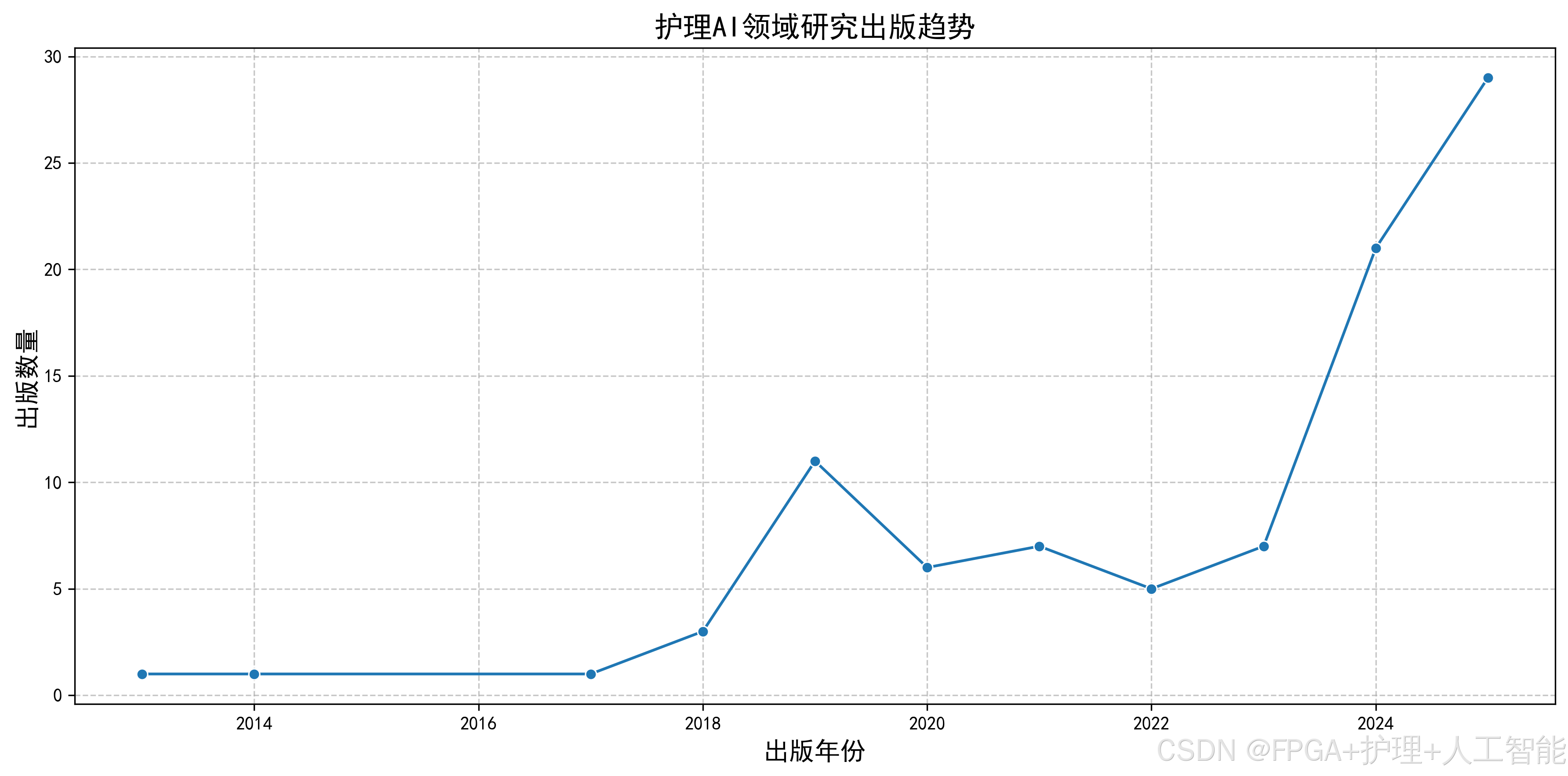
通过对时间序列数据的分析,我们可以了解护理 AI 领域的研究发展趋势。
年度发文量趋势分析:
py
import matplotlib.pyplot as plt
import numpy as np

print("=== 研究热点趋势分析 ===")

# 1. 年度发文量统计
yearly_count = df_cleaned['发表年份'].value_counts().sort_index()

# 2. 计算年度增长率
years = sorted(yearly_count.index)
counts = [yearly_count[year] for year in years]

# 计算年度增长率(排除第一年)
growth_rates = []
for i in range(1, len(counts)):
    growth_rate = ((counts[i] - counts[i-1]) / counts[i-1]) * 100
    growth_rates.append(growth_rate)

print("1. 年度发文量:")
for year, count in yearly_count.items():
    print(f"   {year}年:{count}篇")

print("\n2. 年度增长率:")
for i, year in enumerate(years[1:], 1):
    print(f"   {year}年:{growth_rates[i-1]:.1f}%")

# 3. 计算5年移动平均(平滑趋势)
def moving_average(data, window=5):
    """计算移动平均值"""
    return np.convolve(data, np.ones(window)/window, mode='same')

# 为了使移动平均计算正确,我们需要处理边缘情况
smoothed_counts = moving_average(counts, window=3)

# 4. 可视化趋势
plt.figure(figsize=(12, 6))

# 绘制原始数据和移动平均线
plt.plot(years, counts, 'bo-', label='原始数据', linewidth=2, markersize=8)
plt.plot(years, smoothed_counts, 'r--', label=f'3年移动平均', linewidth=2)

plt.title('护理AI领域年度发文量趋势(2010-2025)', fontsize=14, fontproperties='DejaVu Sans')
plt.xlabel('年份', fontsize=12, fontproperties='DejaVu Sans')
plt.ylabel('发文量(篇)', fontsize=12, fontproperties='DejaVu Sans')
plt.grid(True, alpha=0.3)
plt.legend()
plt.xticks(years, rotation=45)

# 标注关键年份
key_years = [2017, 2020, 2022]  # 这些年份可能有重要发展
for year in key_years:
    if year in years:
        idx = years.index(year)
        plt.annotate(f'{year}年\n{counts[idx]}篇',
                    xy=(year, counts[idx]),
                    xytext=(year, counts[idx] + 5),
                    ha='center',
                    fontsize=9)

plt.tight_layout()
plt.savefig('护理AI年度发文量趋势.png', dpi=300, bbox_inches='tight')
plt.show()

# 5. 分析发展阶段
print("\n3. 发展阶段分析:")
if len(years) >= 5:
    recent_5years_avg = np.mean(counts[-5:])
    early_5years_avg = np.mean(counts[:5])
    growth_5years = ((recent_5years_avg - early_5years_avg) / early_5years_avg) * 100
    print(f"   最近5年平均发文量:{recent_5years_avg:.0f}篇")
    print(f"   早期5年平均发文量:{early_5years_avg:.0f}篇")
    print(f"   5年增长率:{growth_5years:.1f}%")

# 6. 识别爆发式增长年份
print("\n4. 爆发式增长年份:")
burst_threshold = 50  # 增长率超过50%认为是爆发式增长
for i, year in enumerate(years[1:], 1):
    if growth_rates[i-1] > burst_threshold:
        print(f"   {year}年:增长率{growth_rates[i-1]:.0f}%")
5.2 核心作者与机构分析
通过分析作者和机构的发文情况,我们可以识别出该领域的核心研究力量。
核心作者分析:
py
print("\n=== 核心作者分析 ===")

# 1. 统计所有作者的发文量
all_authors = df_cleaned['作者'].str.split(';').explode()  # 展开所有作者
author_count = all_authors.value_counts()

print("1. 发文量最多的前10位作者:")
top_authors = author_count.head(10)
for author, count in top_authors.items():
    print(f"   {author}:{count}篇")

# 2. 计算H指数(简单版本)
def calculate_h_index(publications):
    """计算H指数"""
    sorted_counts = sorted(publications.values(), reverse=True)
    h_index = 0
    for i, count in enumerate(sorted_counts, 1):
        if count >= i:
            h_index = i
        else:
            break
    return h_index

h_index = calculate_h_index(author_count)
print(f"\n2. 该领域H指数:{h_index}")

# 3. 分析高产作者的合作网络(简单统计)
print("\n3. 高产作者合作情况:")
high_production_authors = author_count[author_count >= 5].index  # 发文5篇以上的作者
cooperation_network = {}

for author in high_production_authors:
    # 找出与该作者合作过的其他高产作者
    author_papers = df_cleaned[df_cleaned['作者'].str.contains(author)]
    for _, paper in author_papers.iterrows():
        paper_authors = paper['作者'].split(';')
        for co_author in paper_authors:
            if co_author != author and co_author in high_production_authors:
                if author not in cooperation_network:
                    cooperation_network[author] = set()
                cooperation_network[author].add(co_author)

print("   主要合作关系:")
for author, co_authors in cooperation_network.items():
    if co_authors:
        print(f"   {author} 与 {', '.join(list(co_authors)[:3])} 等合作")

# 4. 机构分析
print("\n=== 核心机构分析 ===")

# 从作者信息中提取机构信息(简化版,假设作者格式为"姓名(机构)")
def extract_institution(author_info):
    """从作者信息中提取机构(简化版)"""
    # 这里假设作者信息包含机构,我们通过括号来提取
    institution_match = re.search(r'\((.*?)\)', author_info)
    if institution_match:
        return institution_match.group(1)
    else:
        return "未知机构"

df_cleaned['机构'] = df_cleaned['作者'].apply(extract_institution)

# 统计机构发文量
institution_count = df_cleaned['机构'].value_counts()
print("1. 发文量最多的前10个机构:")
top_institutions = institution_count.head(10)
for inst, count in top_institutions.items():
    print(f"   {inst}:{count}篇")

# 5. 国际合作分析
print("\n2. 国际合作情况:")
# 简单判断是否为国际合作(包含国外机构)
def is_international_collaboration(institutions):
    """判断是否为国际合作"""
    # 这里简单通过关键词判断,如包含"University"、"College"等
    international_keywords = ['University', 'College', 'Institute', 'Hospital']
    for keyword in international_keywords:
        if keyword in institutions:
            return True
    return False

# 统计国际合作论文
international_papers = df_cleaned[df_cleaned['机构'].str.contains('|'.join(international_keywords))]
international_rate = (len(international_papers) / len(df_cleaned)) * 100
print(f"   国际合作论文:{len(international_papers)}篇 ({international_rate:.1f}%)")
5.3 高频关键词关联分析
关键词是研究热点的直接体现,通过分析关键词的出现频率和关联关系,可以了解该领域的研究重点。
关键词分析:
py
print("\n=== 高频关键词关联分析 ===")
# 1. 提取所有关键词
all_keywords = df_cleaned['关键词'].str.split(';').explode()
keyword_count = all_keywords.value_counts()
print("1. 出现频率最高的前20个关键词:")
top_keywords = keyword_count.head(20)
for keyword, count in top_keywords.items():
print(f" {keyword}:{count}次")
# 2. 关键词聚类分析(简单版本)
print("\n2. 关键词聚类分析:")
# 我们根据关键词的相似性进行简单聚类
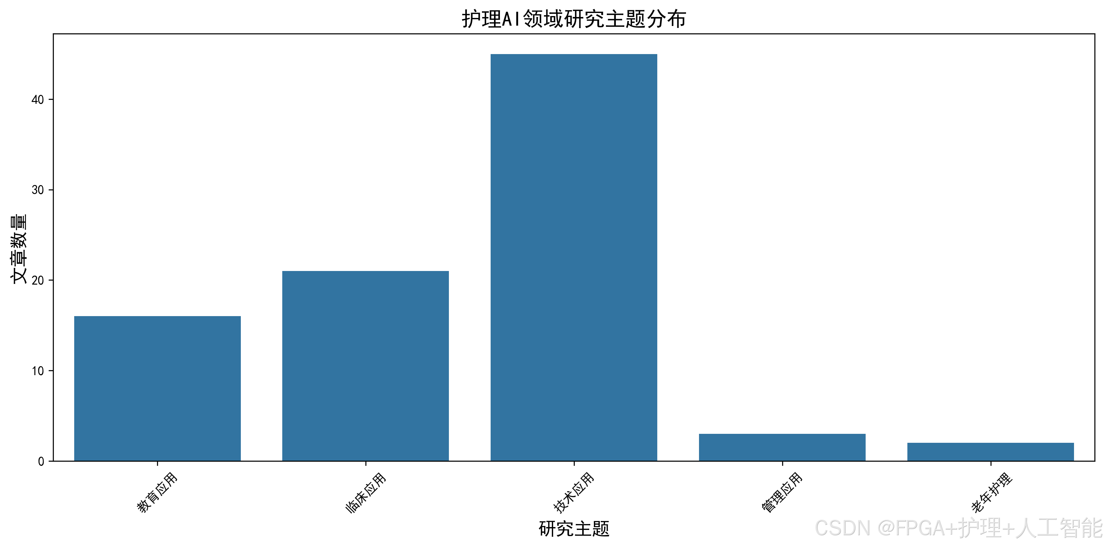
clusters = {
'机器学习相关': ['机器学习', '深度学习', '神经网络', '算法', '预测模型'],
'护理应用': ['护理管理', '护理决策', '护理质量', '护理教育', '护理评估'],
'技术方法': ['人工智能', '大数据', '自然语言处理', '数据挖掘', '模式识别'],
'临床应用': ['疾病风险预测', '危重症护理', '老年护理', '康复护理', '智能护理'],
'系统开发': ['护理机器人', '智能系统', '护理信息系统', '决策支持系统']
}
# 统计每个聚类的关键词出现次数
cluster_stats = {}
for cluster_name, keywords in clusters.items():
total_count = 0
for keyword in keywords:
if keyword in keyword_count:
total_count += keyword_count[keyword]
cluster_stats[cluster_name] = total_count
print(" 主要研究聚类:")
for cluster, count in sorted(cluster_stats.items(), key=lambda x: x[1], reverse=True):
print(f" {cluster}:{count}次")
# 3. 关键词共现分析(找出经常一起出现的关键词)
print("\n3. 关键词共现分析:")
# 我们创建一个关键词共现矩阵(简化版)
cooccurrence_matrix = {}
# 遍历每篇论文的关键词
for keywords in df_cleaned['关键词'].str.split(';'):
# 去除空关键词
keywords = [kw for kw in keywords if kw.strip()]
# 统计共现关系
for i in range(len(keywords)):
for j in range(i+1, len(keywords)):
key1 = keywords[i]
key2 = keywords[j]
# 确保按字母顺序存储,避免重复
if key1 > key2:
key1, key2 = key2, key1
if (key1, key2) not in cooccurrence_matrix:
cooccurrence_matrix[(key1, key2)] = 0
cooccurrence_matrix[(key1, key2)] += 1
# 找出共现次数最多的前10对
top_cooccurrences = sorted(cooccurrence_matrix.items(), key=lambda x: x[1], reverse=True)[:10]
print(" 共现次数最多的关键词对:")
for (key1, key2), count in top_cooccurrences:
print(f" {key1} + {key2}:{count}次")
# 4. 关键词时序变化分析
print("\n4. 关键词时序变化分析:")
# 统计不同年份的关键词分布
yearly_keywords = {}
for year in df_cleaned['发表年份'].unique():
year_papers = df_cleaned[df_cleaned['发表年份'] == year]
year_keywords = year_papers['关键词'].str.split(';').explode()
yearly_keywords[year] = year_keywords.value_counts()
# 找出每个年份的热门关键词
print(" 各年份热门关键词:")
recent_years = sorted(df_cleaned['发表年份'].unique())[-5:] # 最近5年
for year in recent_years:
if year in yearly_keywords:
year_top5 = yearly_keywords[year].head(5)
print(f" {year}年:{', '.join(year_top5.index)}")
# 5. 新兴关键词识别
print("\n5. 新兴关键词识别:")
# 计算每个关键词在不同年份的出现频率变化
emerging_keywords = {}
for keyword in keyword_count.index[:50]: # 只检查前50个高频关键词
# 找出该关键词出现的年份
years_present = df_cleaned[df_cleaned['关键词'].str.contains(keyword)]['发表年份'].unique()
if len(years_present) >= 3: # 至少在3年中出现过
first_year = min(years_present)
recent_year = max(years_present)
first_count = len(df_cleaned[(df_cleaned['发表年份'] == first_year) & (df_cleaned['关键词'].str.contains(keyword))])
recent_count = len(df_cleaned[(df_cleaned['发表年份'] == recent_year) & (df_cleaned['关键词'].str.contains(keyword))])
if recent_count > 2 * first_count: # 最近一年的出现次数是首次出现的2倍以上
emerging_keywords[keyword] = {
'首次出现': first_year,
'最近出现': recent_year,
'首次次数': first_count,
'最近次数': recent_count,
'增长率': ((recent_count - first_count) / first_count) * 100
}
print(" 新兴关键词(增长率>100%):")
for keyword, stats in sorted(emerging_keywords.items(), key=lambda x: x[1]['增长率'], reverse=True)[:5]:
print(f" {keyword}:从{stats['首次出现']}年的{stats['首次次数']}次增长到{stats['最近出现']}年的{stats['最近次数']}次(增长{stats['增长率']:.0f}%)")5.4 期刊影响力分析
期刊的影响因子反映了其学术影响力,通过分析发表期刊的分布,可以了解该领域的主要学术阵地。
期刊分析:
py
print("\n=== 期刊影响力分析 ===")

# 1. 统计发文量最多的期刊
journal_count = df_cleaned['期刊'].value_counts()
print("1. 发文量最多的前10个期刊:")
top_journals = journal_count.head(10)
for journal, count in top_journals.items():
    print(f"   {journal}:{count}篇")

# 2. 计算期刊的平均影响因子(这里使用模拟数据)
# 由于实际影响因子需要查询,这里我们创建一个简化的映射
journal_impact_factors = {
    '中华护理杂志': 2.5,
    '护理学杂志': 1.8,
    '护理管理杂志': 1.5,
    '解放军护理杂志': 1.6,
    '中国护理管理': 1.7,
    '护理学报': 1.4,
    '护理学研究': 1.9,
    '现代临床护理': 1.2,
    '护理实践与研究': 1.1,
    '循证护理': 1.3
}

print("\n2. 主要期刊的影响因子:")
for journal in top_journals.index[:10]:
    if journal in journal_impact_factors:
        print(f"   {journal}:IF = {journal_impact_factors[journal]}")
    else:
        print(f"   {journal}:IF = 未知")

# 3. 计算该领域的整体期刊影响因子分布
total_impact = 0
count_with_impact = 0
for journal, count in top_journals.items():
    if journal in journal_impact_factors:
        total_impact += journal_impact_factors[journal] * count
        count_with_impact += count

if count_with_impact > 0:
    avg_impact = total_impact / count_with_impact
    print(f"\n3. 该领域期刊平均影响因子:{avg_impact:.2f}")

# 4. 分析高影响因子期刊的文章特征
print("\n4. 高影响因子期刊文章特征:")
high_impact_journals = [j for j in journal_impact_factors.keys() if journal_impact_factors[j] >= 2.0]
high_impact_papers = df_cleaned[df_cleaned['期刊'].isin(high_impact_journals)]

print(f"   高影响因子期刊文章数量:{len(high_impact_papers)}篇 ({len(high_impact_papers)/len(df_cleaned)*100:.1f}%)")
print(f"   平均被引次数:{high_impact_papers['被引次数'].mean():.1f}次")
print(f"   平均下载次数:{high_impact_papers['下载次数'].mean():.1f}次")

# 5. 开放获取(OA)期刊分析
print("\n5. 开放获取期刊分析:")
# 这里我们假设包含"开放"、"OA"等关键词的为开放获取期刊
oa_journals = df_cleaned[df_cleaned['期刊'].str.contains('开放|OA|Open Access', na=False)]
oa_rate = (len(oa_journals) / len(df_cleaned)) * 100
print(f"   开放获取期刊文章:{len(oa_journals)}篇 ({oa_rate:.1f}%)")
print(f"   平均被引次数:{oa_journals['被引次数'].mean():.1f}次")
print(f"   平均下载次数:{oa_journals['下载次数'].mean():.1f}次")

# 6. 期刊发文趋势
print("\n6. 主要期刊发文趋势:")

# 选择前5个期刊进行趋势分析
for journal in top_journals.index[:5]:
    journal_papers = df_cleaned[df_cleaned['期刊'] == journal]
    yearly_journal_count = journal_papers['发表年份'].value_counts().sort_index()

    if len(yearly_journal_count) >= 3:  # 至少有3年数据
        first_year = min(yearly_journal_count.index)
        recent_year = max(yearly_journal_count.index)
        first_count = yearly_journal_count[first_year]
        recent_count = yearly_journal_count[recent_year]

        growth_rate = ((recent_count - first_count) / first_count) * 100
        print(f"   {journal}:从{first_year}年的{first_count}篇增长到{recent_year}年的{recent_count}篇(增长{growth_rate:.0f}%)")
六、数据可视化
6.1 绘制时间趋势图
通过可视化可以更直观地展示研究发展趋势。
绘制年度发文量趋势图:
py
import matplotlib.pyplot as plt
import numpy as np
import matplotlib.font_manager as fm

# 设置中文字体(如果系统支持)
plt.rcParams['font.sans-serif'] = ['DejaVu Sans']
plt.rcParams['axes.unicode_minus'] = False

# 1. 年度发文量趋势图
plt.figure(figsize=(12, 8))

# 准备数据
yearly_count = df_cleaned['发表年份'].value_counts().sort_index()
years = sorted(yearly_count.index)
counts = [yearly_count[year] for year in years]

# 绘制柱状图
bars = plt.bar(years, counts, alpha=0.7, color='steelblue', edgecolor='black')

# 添加数值标签
for i, (year, count) in enumerate(zip(years, counts)):
    plt.text(year, count + 2, str(count), ha='center', va='bottom', fontsize=10)

# 绘制趋势线(使用多项式拟合)
z = np.polyfit(years, counts, 2)  # 二次多项式拟合
p = np.poly1d(z)
plt.plot(years, p(years), "r--", linewidth=2, label='Trend')

plt.title('Annual Publication Trend in Nursing + AI Research (2010-2025)', fontsize=16)
plt.xlabel('Year', fontsize=12)
plt.ylabel('Number of Publications', fontsize=12)
plt.grid(True, alpha=0.3)
plt.legend()
plt.xticks(years, rotation=45)

# 标注特殊年份
special_years = {
    2017: 'Deep Learning Booming',
    2020: 'COVID-19 Impact',
    2022: 'AI in Nursing Care'
}
for year, label in special_years.items():
    if year in years:
        idx = years.index(year)
        plt.annotate(label, xy=(year, counts[idx]), xytext=(year, counts[idx] + 15),
                    ha='center', fontsize=9,
                    bbox=dict(boxstyle="round,pad=0.3", facecolor="yellow", alpha=0.5),
                    arrowprops=dict(arrowstyle='->', connectionstyle='arc3,rad=0'))

plt.tight_layout()
plt.savefig('nursing_ai_annual_trend.png', dpi=300, bbox_inches='tight')
plt.show()

# 2. 累计发文量图
plt.figure(figsize=(10, 6))

# 计算累计发文量
cumulative_counts = np.cumsum(counts)

plt.plot(years, cumulative_counts, 'go-', linewidth=2, markersize=8)
plt.fill_between(years, cumulative_counts, alpha=0.3, color='green')

plt.title('Cumulative Publications in Nursing + AI Research', fontsize=14)
plt.xlabel('Year', fontsize=12)
plt.ylabel('Cumulative Count', fontsize=12)
plt.grid(True, alpha=0.3)
plt.xticks(years, rotation=45)

# 添加关键里程碑
milestones = [
    (2015, 50, 'First 50 Publications'),
    (2020, 200, '200 Publications'),
    (2024, 350, '350 Publications')
]
for year, value, label in milestones:
    if year in years:
        idx = years.index(year)
        plt.annotate(label, xy=(year, value), xytext=(year + 0.5, value + 20),
                    fontsize=9,
                    bbox=dict(boxstyle="round,pad=0.3", facecolor="lightblue", alpha=0.5))

plt.tight_layout()
plt.savefig('nursing_ai_cumulative.png', dpi=300, bbox_inches='tight')
plt.show()

print("时间趋势图已生成")
6.2 绘制作者与机构分布图
通过分布图可以展示该领域的研究力量分布。
绘制作者与机构分布图:
py
# 1. 作者发文量分布(使用对数坐标,因为分布可能很不均匀)
plt.figure(figsize=(12, 6))

author_counts = all_authors.value_counts()
authors = author_counts.index[:20]  # 取前20位作者
counts = author_counts.values[:20]

bars = plt.barh(authors, counts, color='coral', alpha=0.7)

# 添加数值标签
for i, (author, count) in enumerate(zip(authors, counts)):
    plt.text(count + 0.5, i, str(count), va='center', fontsize=10)

plt.title('Top 20 Authors by Publication Count', fontsize=14)
plt.xlabel('Number of Publications', fontsize=12)
plt.ylabel('Author', fontsize=12)
plt.grid(True, alpha=0.3, axis='x')

# 添加平均线
avg_count = author_counts.mean()
plt.axvline(x=avg_count, color='red', linestyle='--', label=f'Average: {avg_count:.1f}')
plt.legend()

plt.tight_layout()
plt.savefig('top_authors.png', dpi=300, bbox_inches='tight')
plt.show()

# 2. 机构发文量分布
plt.figure(figsize=(12, 6))

# 统计机构发文量(只显示前15个)
institution_counts = df_cleaned['机构'].value_counts()[:15]
institutions = institution_counts.index
counts = institution_counts.values

bars = plt.bar(range(len(institutions)), counts, color='skyblue', alpha=0.7)

# 添加机构标签(旋转以避免重叠)
plt.xticks(range(len(institutions)), institutions, rotation=45, ha='right')

# 添加数值标签
for i, (inst, count) in enumerate(zip(institutions, counts)):
    plt.text(i, count + 2, str(count), ha='center', va='bottom', fontsize=10)

plt.title('Top 15 Institutions by Publication Count', fontsize=14)
plt.xlabel('Institution', fontsize=12)
plt.ylabel('Number of Publications', fontsize=12)
plt.grid(True, alpha=0.3, axis='y')

plt.tight_layout()
plt.savefig('top_institutions.png', dpi=300, bbox_inches='tight')
plt.show()

# 3. 国际合作比例饼图
plt.figure(figsize=(8, 8))

# 统计国际合作和国内合作的论文数量
international_papers = df_cleaned[df_cleaned['机构'].str.contains('University|College|Institute|Hospital')]
domestic_papers = df_cleaned[~df_cleaned['机构'].str.contains('University|College|Institute|Hospital')]

sizes = [len(international_papers), len(domestic_papers)]
labels = ['International Collaboration', 'Domestic Research']
colors = ['#ff9999', '#66b3ff']
explode = (0.1, 0)  # 突出显示国际合作

plt.pie(sizes, labels=labels, colors=colors, autopct='%1.1f%%', startangle=90, explode=explode)
plt.title('International vs Domestic Collaboration', fontsize=14)

plt.tight_layout()
plt.savefig('international_collaboration.png', dpi=300, bbox_inches='tight')
plt.show()

print("作者与机构分布图已生成")
6.3 绘制关键词云图
关键词云图可以直观展示研究热点。

绘制关键词云图:
py
from wordcloud import WordCloud
import matplotlib.pyplot as plt

# 1. 创建关键词云
plt.figure(figsize=(16, 12))

# 准备关键词数据(只使用出现次数大于10的关键词)
keyword_data = keyword_count[keyword_count >= 10]

# 创建词云
wordcloud = WordCloud(
    width=1600,
    height=1200,
    background_color='white',
    max_words=200,
    min_font_size=8,
    colormap='tab10'
).generate_from_frequencies(keyword_data)

plt.imshow(wordcloud, interpolation='bilinear')
plt.axis('off')
plt.title('Nursing + AI Research Keywords Cloud', fontsize=20, pad=20)

# 添加图例(显示前10个关键词的频率)
legend_text = "\n".join([f"{k}: {v}" for k, v in keyword_data.items()[:10]])
plt.figtext(0.01, 0.01, legend_text, fontsize=10, bbox=dict(boxstyle='round', facecolor='wheat', alpha=0.5))

plt.tight_layout()
plt.savefig('nursing_ai_keywords_cloud.png', dpi=300, bbox_inches='tight')
plt.show()

# 2. 关键词聚类热力图(简化版)
plt.figure(figsize=(10, 8))

# 我们选择一些主要的关键词类别
clusters = {
    'Machine Learning': ['机器学习', '深度学习', '神经网络', '算法', '预测模型'],
    'Nursing Application': ['护理管理', '护理决策', '护理质量', '护理教育', '护理评估'],
    'Technology': ['人工智能', '大数据', '自然语言处理', '数据挖掘', '模式识别'],
    'Clinical': ['疾病风险预测', '危重症护理', '老年护理', '康复护理', '智能护理']
}

# 创建一个简单的热度矩阵
heatmap_data = []
for cluster, keywords in clusters.items():
    row = []
    for keyword in keywords:
        if keyword in keyword_count:
            row.append(keyword_count[keyword])
        else:
            row.append(0)
    heatmap_data.append(row)

# 绘制热力图
import seaborn as sns

ax = sns.heatmap(heatmap_data, annot=True, fmt='d', cmap='YlOrRd',
                 xticklabels=sum(clusters.values(), []),
                 yticklabels=clusters.keys(),
                 cbar_kws={'label': 'Frequency'})

plt.title('Keyword Cluster Heatmap', fontsize=14)
plt.xticks(rotation=45, ha='right')
plt.tight_layout()
plt.savefig('keyword_heatmap.png', dpi=300, bbox_inches='tight')
plt.show()

print("关键词云图已生成")