已知一个函数的图像,通过适当的变换,得到另一个与之相关的函数的图像,这样的绘图方法叫做图像变换,常用的图像变换是平移变换、对称变换 和 伸缩变换。
一、 平移变换
1. 左平移
将函数 y = f(x) 向左平移 m( m > 0) 个单位长度, 得到函数 y = f(x + m) 的图像,如下
Python代码:
python
import matplotlib.pyplot as plt
import numpy as np
from test0 import create_coordinate_system

# 创建一个坐标系
fig, ax = create_coordinate_system(x_range=(-10, 10), y_range=(-4, 10), figsize=(8, 6))

# 添加一个二次函数的图像
x = np.linspace(0.5, 5.5, 100)
y = (x-3)**2 - 2

# 向左平移6个单位,(x - 3) + 6 = x + 3
x1 = np.linspace(-5.5, -0.5, 100)
y1 = (x1+3)**2 - 2

# 绘制二次函数的图像
ax.plot(x, y, 'r-', linewidth=2, label='y = f(x)', color='black')
ax.plot(x1, y1, 'r-', linewidth=2, label='y = f(x+m)', color='red')
ax.legend()
plt.show()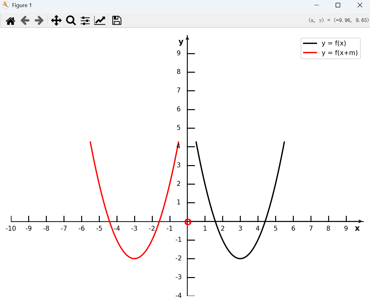
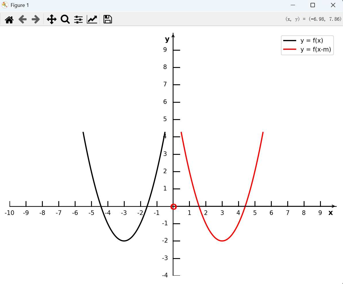
2. 右平移
将函数 y = f(x) 向右平移 m( m > 0) 个单位长度, 得到函数 y = f(x - m) 的图像,如下
Python代码:
python
import matplotlib.pyplot as plt
import numpy as np
from test0 import create_coordinate_system

# 创建一个坐标系
fig, ax = create_coordinate_system(x_range=(-10, 10), y_range=(-4, 10), figsize=(8, 6))

# 添加一个二次函数的图像
x = np.linspace(-5.5, -0.5, 100)
y = (x+3)**2 - 2

# 向右平移6个单位,(x + 3) - 6 = x - 3
x1 = np.linspace(0.5, 5.5, 100)
y1 = (x1-3)**2 - 2

# 绘制二次函数的图像
ax.plot(x, y, 'r-', linewidth=2, label='y = f(x)', color='black')
ax.plot(x1, y1, 'r-', linewidth=2, label='y = f(x-m)', color='red')
ax.legend()
plt.show()
运行结果:
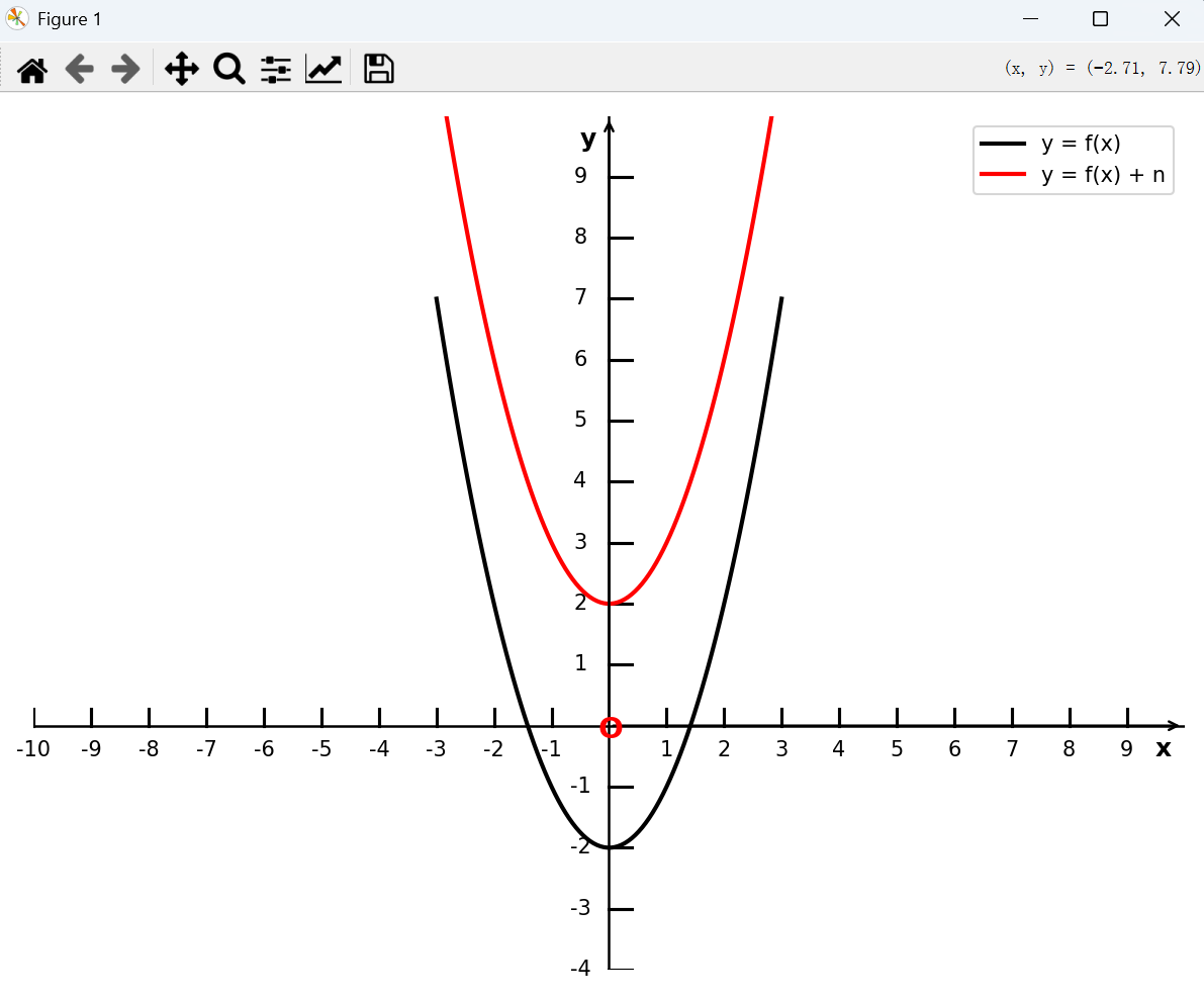
3. 上平移
将函数 y = f(x) 向上平移 n( n > 0) 个单位长度, 得到函数 y = f(x) + n 的图像,如下
Python 代码:
python
import matplotlib.pyplot as plt
import numpy as np
from test0 import create_coordinate_system

# 创建一个坐标系
fig, ax = create_coordinate_system(x_range=(-10, 10), y_range=(-4, 10), figsize=(8, 6))

# 添加一个二次函数的图像
x = np.linspace(-3, 3, 100)
y = x**2 - 2

# 向上移动4个单位,-2 + 4 = 2
x1 = np.linspace(-3, 3, 100)
y1 = x1**2 + 2

# 绘制二次函数的图像
ax.plot(x, y, 'r-', linewidth=2, label='y = f(x)', color='black')
ax.plot(x1, y1, 'r-', linewidth=2, label='y = f(x) + n', color='red')

ax.legend()
plt.show()
运行结果:
4. 下平移
将函数 y = f(x) 向左平移 n( n > 0) 个单位长度, 得到函数 y = f(x) - n 的图像,如下
Python代码:
python
import matplotlib.pyplot as plt
import numpy as np
from test0 import create_coordinate_system

# 创建一个坐标系
fig, ax = create_coordinate_system(x_range=(-10, 10), y_range=(-4, 10), figsize=(8, 6))
# 添加一个二次函数的图像
x = np.linspace(-3, 3, 100)
y = x**2 + 2

# 向下移动4个单位,2 - 4 = -2
x1 = np.linspace(-3, 3, 100)
y1 = x1**2 - 2

# 绘制二次函数的图像
ax.plot(x, y, 'r-', linewidth=2, label='y = f(x)', color='black')
ax.plot(x1, y1, 'r-', linewidth=2, label='y = f(x) - n', color='red')
ax.legend()
plt.show()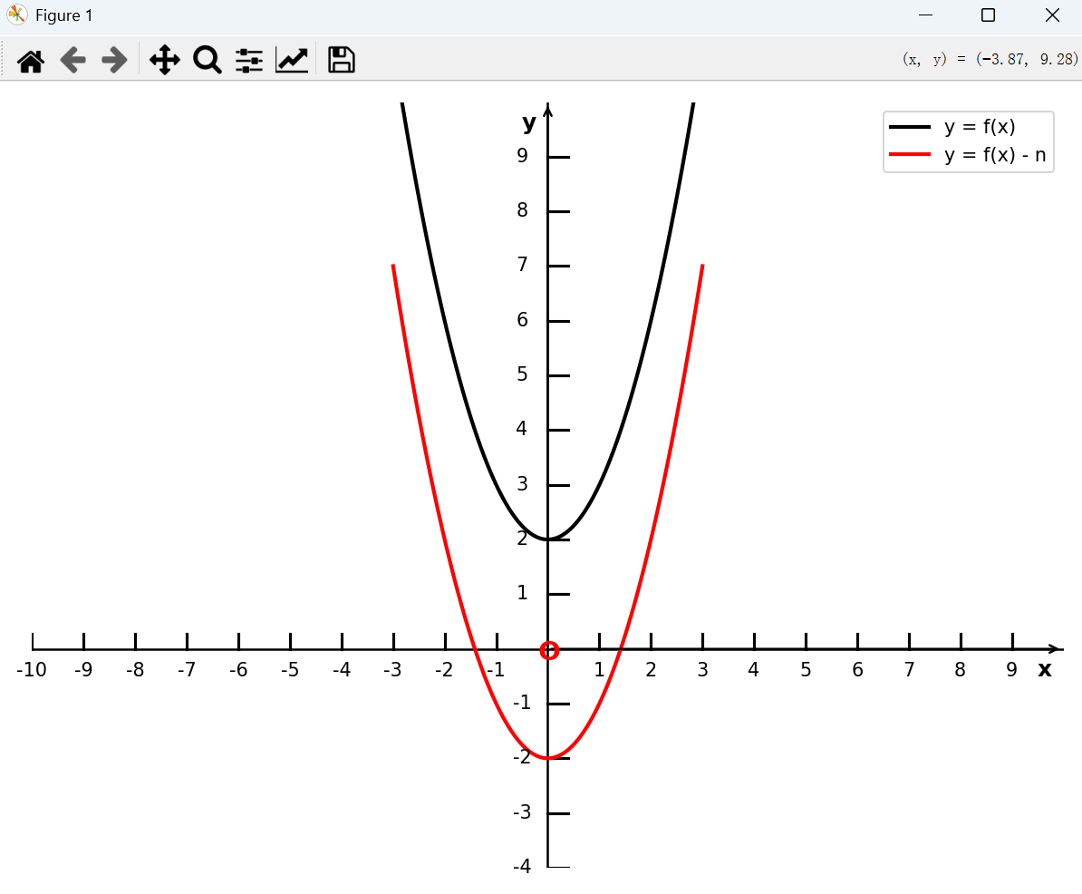
二、 对称变换
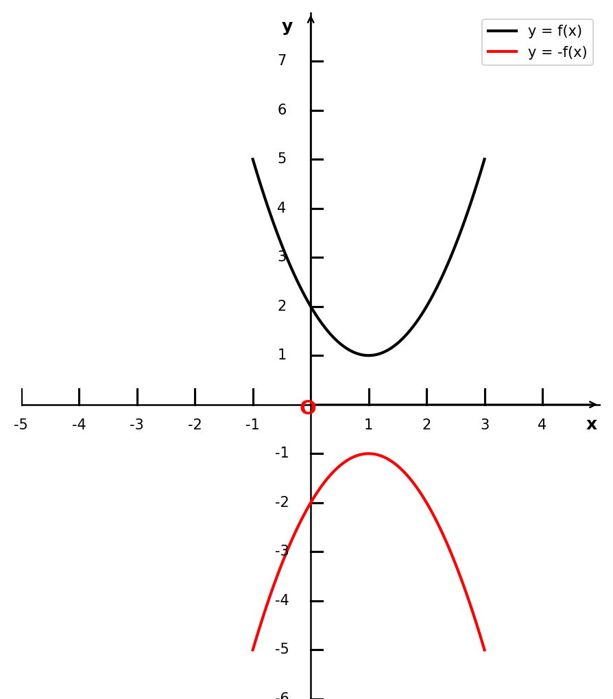
1. 关于x轴对称
将函数 y = f(x) 的图像关于 x 轴对称,得到函数 y = -f(x) 的图像
Python代码:
python
import matplotlib.pyplot as plt
import numpy as np
from test0 import create_coordinate_system

# 创建一个坐标系
fig, ax = create_coordinate_system(x_range=(-5, 5), y_range=(-8, 8), figsize=(6, 8))

# 添加一个二次函数的图像
x = np.linspace(-1, 3, 100)
y = (x-1)**2 + 1
# 关于X轴对称,-((x-1)**2 + 1) = -(x-1)**2 - 1
x1 = np.linspace(-1, 3, 100)
y1 = -(x1-1)**2 - 1

# 绘制二次函数的图像
ax.plot(x, y, 'r-', linewidth=2, label='y = f(x)', color='black')
ax.plot(x1, y1, 'r-', linewidth=2, label='y = -f(x)', color='red')

ax.legend()
plt.show()
运行结果:
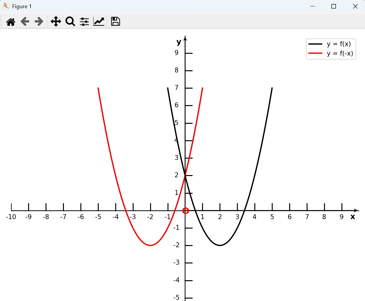
2. 关于y轴对称
将函数 y = f(x) 的图像关于 y 轴对称,得到函数 y = f(-x) 的图像
Python代码:
python
import matplotlib.pyplot as plt
import numpy as np
from test0 import create_coordinate_system

# 创建一个坐标系
fig, ax = create_coordinate_system(x_range=(-10, 10), y_range=(-10, 10), figsize=(8, 8))

# 添加一个二次函数的图像
x = np.linspace(-1, 5, 100)
y = (x-2)**2 - 2

# 关于Y轴对称,(-x-2)**2 = (x+2)**2
x1 = np.linspace(-5, 1, 100)
y1 = (x1+2)**2 - 2

# 绘制二次函数的图像
ax.plot(x, y, 'r-', linewidth=2, label='y = f(x)', color='black')
ax.plot(x1, y1, 'r-', linewidth=2, label='y = f(-x)', color='red')
ax.legend()
plt.show()
运行结果:
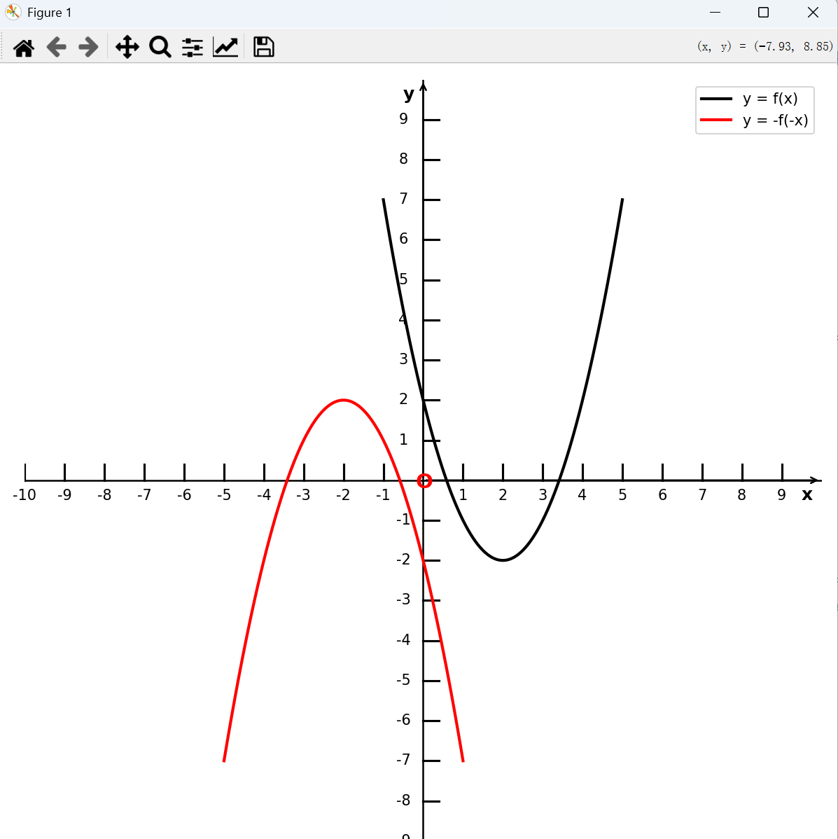
3. 关于原点对称
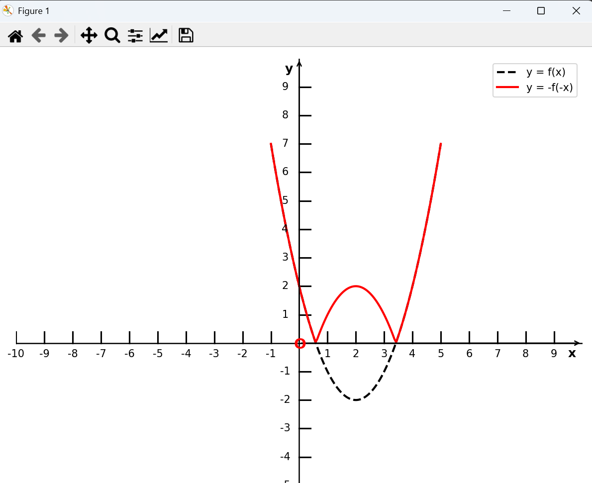
将函数 y = f(x) 的图像关于原点对称,得到函数 y = -f(-x) 的图像
Python代码:
python
import matplotlib.pyplot as plt
import numpy as np
from test0 import create_coordinate_system

# 创建一个坐标系
fig, ax = create_coordinate_system(x_range=(-10, 10), y_range=(-10, 10), figsize=(8, 8))

# 添加一个二次函数的图像
x = np.linspace(-1, 5, 100)
y = (x-2)**2 - 2

# 关于Y轴对称,-((-x-2)**2 -2) = 2-(x+2)**2
x1 = np.linspace(-5, 1, 100)
y1 = 2-(x1+2)**2
# 绘制二次函数的图像
ax.plot(x, y, 'r-', linewidth=2, label='y = f(x)', color='black')
ax.plot(x1, y1, 'r-', linewidth=2, label='y = -f(-x)', color='red')
ax.legend()
plt.show()
运行结果:
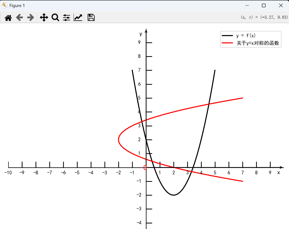
4. 关于执行 y = x 对称
将函数 y = f(x) 的图像关于直线 y = x 对称,得到函数 y=f−1(x)y = f^-1(x)y=f−1(x) 的图像
Python代码:
python
import matplotlib.pyplot as plt
import numpy as np
from test0 import create_coordinate_system

# 支持中文
plt.rcParams['font.family'] = ['sans-serif']
plt.rcParams['font.sans-serif'] = ['SimHei']

# 创建一个坐标系
fig, ax = create_coordinate_system(x_range=(-10, 10), y_range=(-10, 10), figsize=(8, 8))

# 添加一个二次函数的图像
x = np.linspace(-1, 5, 100)
y = (x-2)**2 - 2
# x 和 y 互换
x1 = y
y1 = x
# 绘制二次函数的图像
ax.plot(x, y, 'r-', linewidth=2, label='y = f(x)', color='black')
ax.plot(x1, y1, 'r-', linewidth=2, label='关于y=x对称的函数', color='red')
ax.legend()
plt.show()
运行结果:
5. 将x轴下方对称到x轴上方
保留函数 y = f(x) 在 x 轴及 x 轴上方的部分, 把 x 轴下方的部分关于 x 轴对称到 x 轴上方(去掉原来下方的部分), 得到函数 y = |f(x)| 的图像
Python 代码:
python
import matplotlib.pyplot as plt
import numpy as np
from test0 import create_coordinate_system

# 创建一个坐标系
fig, ax = create_coordinate_system(x_range=(-10, 10), y_range=(-10, 10), figsize=(8, 8))
# 添加一个二次函数的图像
x = np.linspace(-1, 5, 100)
y = (x-2)**2 - 2

# y = |f(x)|
x1 = np.linspace(-1, 5, 100)
y1 = abs((x1-2)**2 - 2)
# 绘制二次函数的图像
ax.plot(x, y, 'r-', linewidth=2, label='y = f(x)', color='black', linestyle='--')
ax.plot(x1, y1, 'r-', linewidth=2, label='y = -f(-x)', color='red')
ax.legend()
plt.show()
运行结果:
6. y轴右边对称到y轴左边
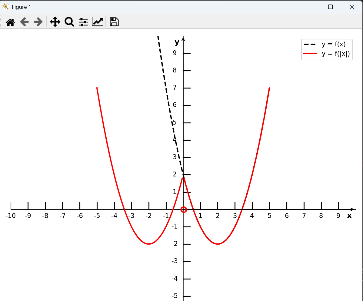
保留函数 y = f(x) 在y轴及y轴右侧的部分,去掉 y 轴左侧的部分,再将 y 轴右侧图像对称到 y 轴左侧,得到函数 y = f(|x|) 的图像
Python代码:
python
import matplotlib.pyplot as plt
import numpy as np
from test0 import create_coordinate_system

# 创建一个坐标系
fig, ax = create_coordinate_system(x_range=(-10, 10), y_range=(-10, 10), figsize=(8, 8))
# 添加一个二次函数的图像
x = np.linspace(-5, 5, 100)
y = (x-2)**2 - 2
# y = f(|x|)
x1 = np.linspace(-5, 5, 100)
y1 = (abs(x1)-2)**2 - 2

# 绘制二次函数的图像
ax.plot(x, y, 'r-', linewidth=2, label='y = f(x)', color='black', linestyle='--')
ax.plot(x1, y1, 'r-', linewidth=2, label='y = f(|x|)', color='red')
ax.legend()
plt.show()
运行结果:
三、伸缩变换
1. 水平伸缩
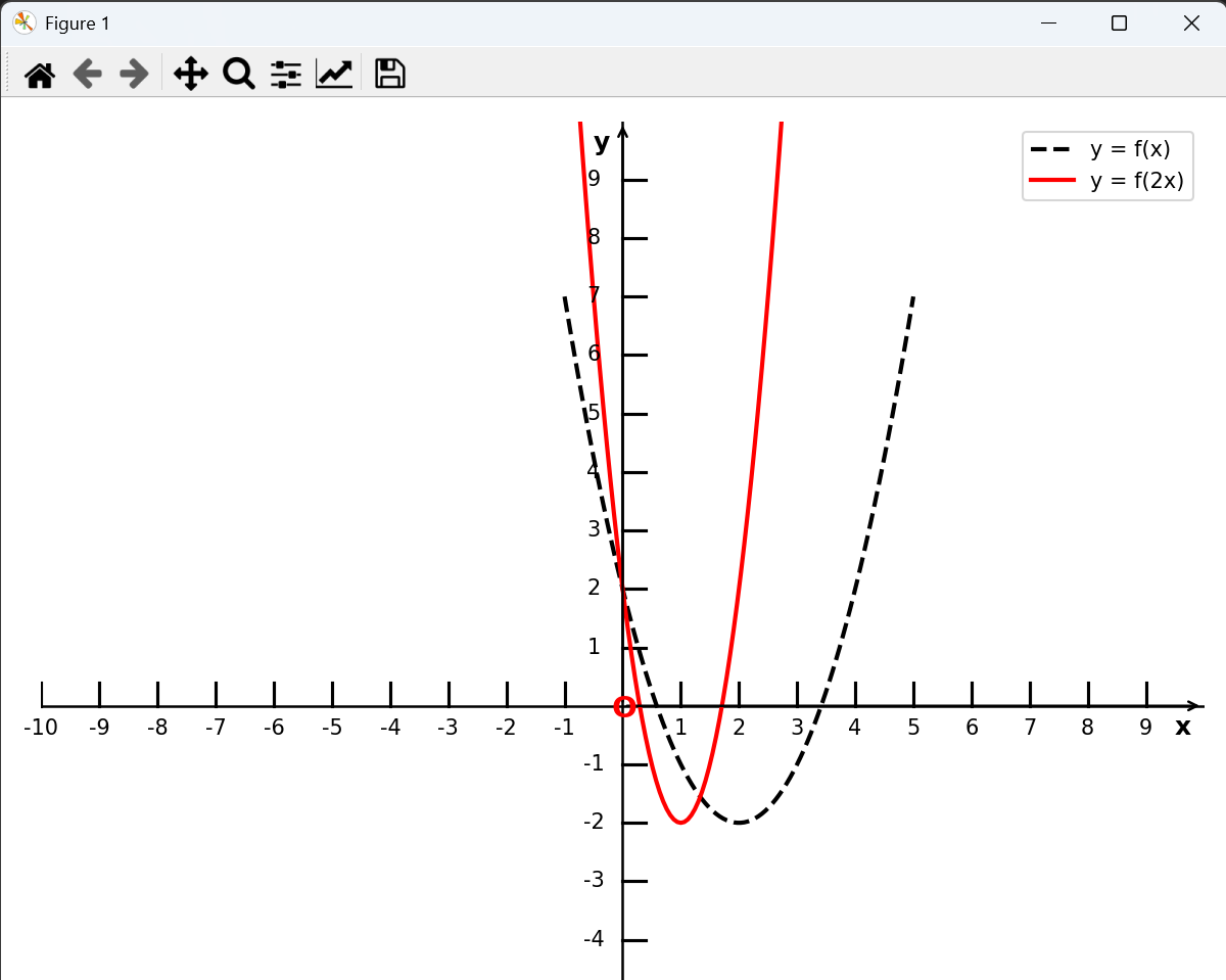
y = f(wx)(w > 1)的图像, 可由 y = f(x) 的图像上每点的横坐标缩短到原来的 1/w 倍(纵坐标不变)得到;
y = f(wx)(0 < w < 1)的图像,可由 y = f(x) 的图像上每点的横坐标伸长到原来的 1/w 倍(纵坐标不变)得到;
Python代码:
python
import matplotlib.pyplot as plt
import numpy as np
from test0 import create_coordinate_system

# 创建一个坐标系
fig, ax = create_coordinate_system(x_range=(-10, 10), y_range=(-10, 10), figsize=(8, 8))

# 添加一个二次函数的图像
x = np.linspace(-1, 5, 100)
y = (x-2)**2 - 2

# y = f(2x) 横坐标缩小为1/2倍
x1 = np.linspace(-1, 5, 100)
y1 = (2*x1-2)**2 - 2

# 绘制二次函数的图像
ax.plot(x, y, 'r-', linewidth=2, label='y = f(x)', color='black', linestyle='--')
ax.plot(x1, y1, 'r-', linewidth=2, label='y = f(2x)', color='red')
ax.legend()
plt.show()
运行结果:
2. 垂直伸缩
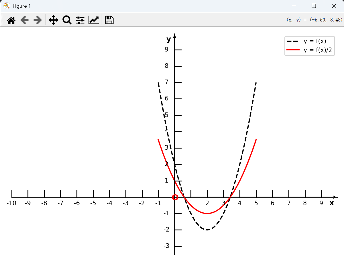
y = Af(wx)(A > 1)的图像, 可由 y = f(x) 的图像上每点的纵坐标伸长到原来的 A 倍(横坐标不变)得到;
y = Af(wx)(0 < A < 1)的图像, 可由 y = f(x) 的图像上每点的纵坐标缩短到原来的 A 倍(横坐标不变)得到;
Python代码:
python
import matplotlib.pyplot as plt
import numpy as np
from test0 import create_coordinate_system
# 创建一个坐标系
fig, ax = create_coordinate_system(x_range=(-10, 10), y_range=(-10, 10), figsize=(8, 8))
# 添加一个二次函数的图像
x = np.linspace(-1, 5, 100)
y = (x-2)**2 - 2
# y = f(x)/2 纵坐标缩小为1/2倍
x1 = np.linspace(-1, 5, 100)
y1 = (1/2)*((x-2)**2 - 2)
# 绘制二次函数的图像
ax.plot(x, y, 'r-', linewidth=2, label='y = f(x)', color='black', linestyle='--')
ax.plot(x1, y1, 'r-', linewidth=2, label='y = f(x)/2', color='red')
ax.legend()
plt.show()
执行结果:
三、总结
后续我将继续使用Python实现扈志明《微积分》教材中的更多内容,包括极限、导数、积分等核心概念,通过编程实践深化对微积分知识的理解。
参考教材:扈志明,《微积分》,高等教育出版社。本文中的数学定义和概念均来源于此教材。