牛客网 AI题（一）机器学习 + 深度学习

[深度学习 DL](#深度学习 DL)

[DL4 Log Softmax函数的实现](#DL4 Log Softmax函数的实现)

[DL7 两个正态分布之间的KL散度](#DL7 两个正态分布之间的KL散度)

[DL15 实现自注意力机制](#DL15 实现自注意力机制)

[DL16 RNN 简化版](#DL16 RNN 简化版)

[DL17 实现长短期记忆（LSTM）网络](#DL17 实现长短期记忆（LSTM）网络)

[机器学习 ML](#机器学习 ML)

[ML2 使用梯度下降的线性回归](#ML2 使用梯度下降的线性回归)

[ML3 标准化缩放和最大最小缩放](#ML3 标准化缩放和最大最小缩放)

[ML5 损失函数](#ML5 损失函数)

[ML6 鸢尾花分类](#ML6 鸢尾花分类)

深度学习 DL

DL4 Log Softmax函数的实现

先减去最大值，再对softmax 结果取log

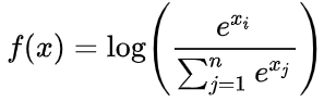
题目让返回 np.ndarray 的结果，先转化为 np.array() 利用 numpy 的广播性。

python 复制代码

import numpy as np
def log_softmax(scores: list) -> np.ndarray:
    arr = np.array(scores)
    arr = arr - np.max(arr)
    return arr - np.log(sum(np.exp(arr)))

if __name__ == "__main__":
    scores = eval(input())
    print(log_softmax(scores))

DL7 两个正态分布之间的KL散度

KL散度衡量两个分布的差异

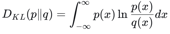
对于正态分布：

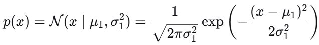
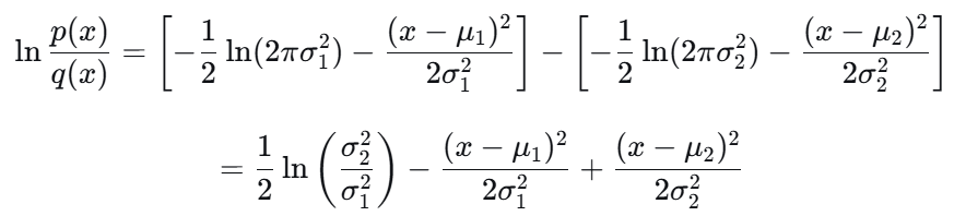
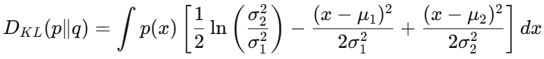
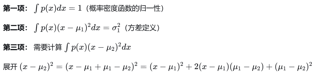
最终结果：

DL15 实现自注意力机制

复制代码

# Q: [序列长度, 特征维度], K: [序列长度, 特征维度]
# scores = Q @ K.T / sqrt(d_k)  →  [序列长度, 序列长度]

得到矩阵：每个位置对其他位置的注意力分数（n*n矩阵）；

对每行（每个token对其他）softmax（axis = 0 竖着一列操作；axis = 1 横着一行操作）

在sum求和的时候，会把 (n*n)的矩阵变成长度为n的向量，删掉一维，导致除法维度不对应。

keepdims=True，使得最后一维保留为1，变成 (n,1)。

python 复制代码

import numpy as np

def compute_qkv(X, W_q, W_k, W_v):
    return X @ W_q, X @ W_k, X @ W_v

def self_attention(Q, K, V):
    # Q * K
    d_k = np.sqrt(Q.shape[1]) # 缩放点积，防止梯度消失
    scores = Q @ K.T / d_k
    # softmax 并对求和保持后一维度
    weights = np.exp(scores) / np.sum(np.exp(scores), axis=1, keepdims=True)
    return weights @ V


if __name__ == "__main__":
    X = np.array(eval(input()))
    W_q = np.array(eval(input()))
    W_k = np.array(eval(input()))
    W_v = np.array(eval(input()))
    Q, K, V = compute_qkv(X, W_q, W_k, W_v)
    print(self_attention(Q, K, V))

DL16 RNN 简化版

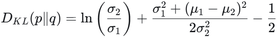
简化版题：给定Wx，Wh，b；最初的h以及从前到后的 input_sequence

只要求最后的隐藏层 h；

python 复制代码

def rnn_forward(input_sequence, h, Wx, Wh, b):
    for x in input_sequence:
        h = np.tanh(np.dot(Wx,x) + np.dot(Wh,h) + b)
    return np.round(h, 4).tolist()

DL17 实现长短期记忆（LSTM）网络

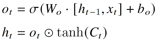
三态门 + 细胞状态 => 隐状态 h；处理时将前一个h和x 拼在一起。

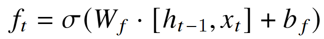
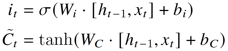
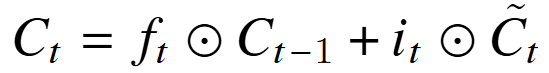
新细胞状态C：遗忘门 f 和输入门 i；对之前与候选细胞状态进行加权。

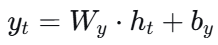
输出门并更新隐状态 h。

python 复制代码

def sigmoid(self, x):
	return 1 / (1 + np.exp(-x))

def forward(self, x, h, c):
    outputs = []
    for t in range(len(x)):
        # 拿出t时间的x转化为列向量 最后一列加上xt变为 (h,xt)
        xt = x[t].reshape(-1,1)
        concat = np.vstack((h, xt))

        # 遗忘门
        ft = self.sigmoid(np.dot(self.Wf, concat) + self.bf)

        # 输入门
        it = self.sigmoid(np.dot(self.Wi, concat) + self.bi)
        c_tilde = np.tanh(np.dot(self.Wc, concat) + self.bc)

        # 细胞状态更新
        c = ft * c + it * c_tilde

        # 输出门
        ot = self.sigmoid(np.dot(self.Wo, concat) + self.bo)

        # 隐状态更新
        h = ot * np.tanh(c)

        outputs.append(h)

    return np.array(outputs), h, c

机器学习 ML

ML2 使用梯度下降的线性回归

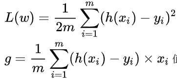h(x) = x @ θ

| 步骤 | 运算 | 输入形状 | 输出形状 |
| 预测 | X @ theta | (m,n)@(n,1) | (m,1) |
| 误差 | predictions - y | (m,1)-(m,1) | (m,1) |
| 梯度 | X.T @ errors | (n,m)@(m,1) | (n,1) |

更新	theta - α×updates	(n,1)-(n,1)	(n,1)

python 复制代码

import numpy as np
def linear_regression_gradient_descent(X, y, alpha, iterations):
    m, n = X.shape
    theta = np.zeros((n,1))
    for _ in range(iterations):
        pre = X @ theta
        errors = pre - y.reshape(-1,1) # 把y变成列向量
        theta -= alpha * (X.T @ errors) / m
    return np.round(theta.flatten(),4) # 把(n,1)二维的拉直为 长度为n的列表

ML3 标准化缩放和最大最小缩放

对每列进行两种缩放。 axis = 0 并广播机制。

python 复制代码

def feature_scaling(data):
    # 标准化
    mean = np.mean(data, axis=0)
    std = np.std(data, axis=0)
    standardized_data = (data - mean) / std
     
    # 最大最小
    min_val = np.min(data, axis=0)
    max_val = np.max(data, axis=0)
    normalized_data = (data - min_val) / (max_val - min_val)
     
    return np.round(standardized_data,4).tolist(), np.round(normalized_data,4).tolist()

sklearn 版本预处理库的两种Scaler

python 复制代码

def feature_scaling(data):
    from sklearn.preprocessing import StandardScaler, MinMaxScaler
    return np.round(StandardScaler().fit_transform(data),4).tolist(), np.round(MinMaxScaler().fit_transform(data),4).tolist()

ML5 损失函数

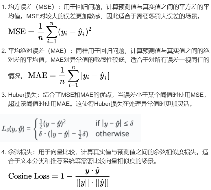
numpy的使用，mse mae 按规则计算取平均 np.mean()

np.where起到条件选择的作用；np.dot np.norm 进行点积和二范数

python 复制代码

import numpy as np
def calculate_loss(real, pre, delta):
    mse = np.mean((real-pre)**2)
    mae = np.mean(np.abs(real-pre))
    huber_loss = np.where(np.abs(real-pre)<=delta, mse, mae)
    cosine_loss = 1 - np.dot(real,pre) / np.linalg.norm(real) / np.linalg.norm(pre)
    return round(mse, 6), round(mae, 6), round(np.mean(huber_loss), 6), round(cosine_loss, 6)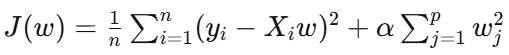

M11 岭回归损失函数

python 复制代码

# 岭回归
def ridge_loss(X, w, y_true, alpha):
    return np.mean( (y_true-X@w)**2 ) + alpha*np.sum(w**2)

ML7 数据集洗牌 np.random.shuffle

对索引 [0,n) 进行shuffle洗牌；对np.random 设定随机种子

python 复制代码

import numpy as np

def shuffle_data(X, y, seed=None):
    if seed:
        np.random.seed(seed) # 为np.random 设定随机种子
    # 索引shuffle
    idx = np.arange(X.shape[0])
    np.random.shuffle(idx)
    return X[idx], y[idx]
    
    
if __name__ == "__main__":
    X = np.array(eval(input()))
    y = np.array(eval(input()))
    print(shuffle_data(X, y, 42))

ML6 鸢尾花分类

你的任务是用sklearn的LogisticsRegression模型对鸢尾花类别进行预测，模型请指定参数max_iter=200以减少训练用时。

1.读入数据集

2.对数据集进行一次随机洗牌（索引顺序shuffle）

3.数据分成训练集与测试集（后n为测试）

输出预测类别；最大概率。

分别用predict 和 predict_proba。

python 复制代码

from sklearn.datasets import load_iris
from sklearn.linear_model import LogisticRegression
import numpy as np
import random 

iris = load_iris()
X = iris.data
y = iris.target

n = int(input())

random.seed(42)

indices = list(range(len(X)))  # 创建索引列表
random.shuffle(indices)  # 洗牌
X = X[indices]  # 根据洗牌后的索引重新排列数据
y = y[indices]  # 根据洗牌后的索引重新排列标签
 
X_train, X_test, y_train, y_test = X[:-n], X[-n:], y[:-n], y[-n:]

 
# 3. 使用逻辑回归算法进行训练
model = LogisticRegression(max_iter=200)
model.fit(X_train, y_train)
 
# 4. 进行预测
y_pred = model.predict(X_test)
y_prob = model.predict_proba(X_test)

# 5. 输出预测的类别以及对应的概率
for i in range(len(y_pred)):
    print(f'{iris.target_names[y_pred[i]]} {y_prob[i][y_pred[i]]:.2f}')