快速上手大模型:机器学习3(多元线性回归及梯度、向量化、正规方程)

目录

[1 多元线性回归(Multiple liner regression)](#1 多元线性回归(Multiple liner regression))

[1.1 定义](#1.1 定义)

[2 向量化](#2 向量化)

[2.1 例子](#2.1 例子)

[2.2 代码实现](#2.2 代码实现)

[2.3 NumPy规则](#2.3 NumPy规则)

[2.4 向量点积运算(dot product multiplies the values)](#2.4 向量点积运算(dot product multiplies the values))

[2.5 矩阵创建](#2.5 矩阵创建)

[2.6 矩阵索引](#2.6 矩阵索引)

[3 多元线性回归的梯度下降法](#3 多元线性回归的梯度下降法)

[3.1 定义](#3.1 定义)

[3.2 梯度函数](#3.2 梯度函数)

[4 正规方程(Normal equation)求解代价函数](#4 正规方程(Normal equation)求解代价函数)

[4.1 定义](#4.1 定义)

[4.2 缺点](#4.2 缺点)


学习目的:

让线性回归更快、更强大。

1 多元线性回归(Multiple liner regression)

1.1 定义

:第j个特征;

n:特征总数;

:第i个训练样本的所有特征;

:第j个特征第i个训练样本。

多元线性回归 (Multiple liner regression):多个输入特征的线性回归模型,表达式

2 向量化

2.1 例子

向量化使代码简洁、运行高效。

2.2 代码实现

使用Python编译,调用NumPy包
(1)引入模块/包

复制代码
import numpy as np    # it is an unofficial standard to use np for numpy
import time

(2)数组创建

代码:

复制代码
# NumPy routines which allocate memory and fill arrays with value
a = np.zeros(4);                print(f"np.zeros(4) :   a = {a}, a shape = {a.shape}, a data type = {a.dtype}")
a = np.zeros((4,));             print(f"np.zeros(4,) :  a = {a}, a shape = {a.shape}, a data type = {a.dtype}")
a = np.random.random_sample(4); print(f"np.random.random_sample(4): a = {a}, a shape = {a.shape}, a data type = {a.dtype}")

输出:

复制代码
# NumPy routines which allocate memory and fill arrays with value
a = np.zeros(4);                print(f"np.zeros(4) :   a = {a}, a shape = {a.shape}, a data type = {a.dtype}")
a = np.zeros((4,));             print(f"np.zeros(4,) :  a = {a}, a shape = {a.shape}, a data type = {a.dtype}")
a = np.random.random_sample(4); print(f"np.random.random_sample(4): a = {a}, a shape = {a.shape}, a data type = {a.dtype}")

np.zeros(4):创建一个长度为4的数组,所有元素都是 0.0(浮点数);

a.shape:数组形状,这里是 (4,),表示一维数组长度 4;

a.dtype:数据类型。

2.3 NumPy规则

(1)索引(Indexing)

负的从末尾去找,超限报错。

例子:

复制代码
#vector indexing operations on 1-D vectors
a = np.arange(10)
print(a)

#access an element
print(f"a[2].shape: {a[2].shape} a[2]  = {a[2]}, Accessing an element returns a scalar")

# access the last element, negative indexes count from the end
print(f"a[-1] = {a[-1]}")

#indexs must be within the range of the vector or they will produce and error
try:
    c = a[10]
except Exception as e:
    print("The error message you'll see is:")
    print(e)

输出:

复制代码
[0 1 2 3 4 5 6 7 8 9]
a[2].shape: () a[2]  = 2, Accessing an element returns a scalar
a[-1] = 9
The error message you'll see is:
index 10 is out of bounds for axis 0 with size 10

(2)切片(Slicing)

复制代码
a[start : stop : step]

start:起始索引,包含起始;

stop:终止索引,不包含终止位;

step:步长,每隔多少取一个。

例子:

复制代码
#vector slicing operations
a = np.arange(10)
print(f"a         = {a}")

# access all elements index 3 and above
c = a[3:];        print("a[3:]    = ", c)

# access all elements below index 3
c = a[:3];        print("a[:3]    = ", c)

# access all elements
c = a[:];         print("a[:]     = ", c)

输出:

复制代码
a[3:]    =  [3 4 5 6 7 8 9]
a[:3]    =  [0 1 2]
a[:]     =  [0 1 2 3 4 5 6 7 8 9]
2.4 向量点积运算(dot product multiplies the values)

代码:

复制代码
import numpy as np

# test 1-D
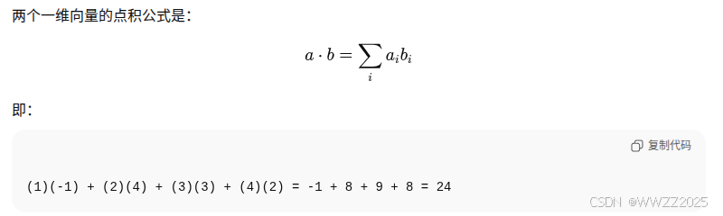
a = np.array([1, 2, 3, 4])
b = np.array([-1, 4, 3, 2])
c = np.dot(a, b)
print(f"NumPy 1-D np.dot(a, b) = {c}, np.dot(a, b).shape = {c.shape} ") 
c = np.dot(b, a)
print(f"NumPy 1-D np.dot(b, a) = {c}, np.dot(a, b).shape = {c.shape} ")

输出:

复制代码
# np.dot(a, b).shape = () 此处输出为空,因为np.dot(a, b)是数值,不存在维度说法
NumPy 1-D np.dot(a, b) = 24, np.dot(a, b).shape = () 
NumPy 1-D np.dot(b, a) = 24, np.dot(a, b).shape = () 
2.5 矩阵创建

代码:

复制代码
a = np.zeros((1, 5))                                       
print(f"a shape = {a.shape}, a = {a}")                     

a = np.zeros((2, 1))                                                                   
print(f"a shape = {a.shape}, a = {a}") 

a = np.random.random_sample((1, 1))  
print(f"a shape = {a.shape}, a = {a}") 

输出:

复制代码
a = np.zeros((1, 5))                                       
print(f"a shape = {a.shape}, a = {a}")                     

a = np.zeros((2, 1))                                                                   
print(f"a shape = {a.shape}, a = {a}") 

a = np.random.random_sample((1, 1))  
print(f"a shape = {a.shape}, a = {a}") 
2.6 矩阵索引

代码:

复制代码
#vector indexing operations on matrices
"""np.arange(6) → 生成一个一维数组 [0, 1, 2, 3, 4, 5]
   .reshape(-1, 2) → 重新调整形状为 N×2 的矩阵
   这里的 -1 表示 自动计算行数,使总元素数量不变。"""
a = np.arange(6).reshape(-1, 2)   #reshape is a convenient way to create matrices
print(f"a.shape: {a.shape}, \na= {a}")

#access an element
print(f"\na[2,0].shape:   {a[2, 0].shape}, a[2,0] = {a[2, 0]},     type(a[2,0]) = {type(a[2, 0])} Accessing an element returns a scalar\n")

#access a row
print(f"a[2].shape:   {a[2].shape}, a[2]   = {a[2]}, type(a[2])   = {type(a[2])}")

输出:

复制代码
a.shape: (3, 2), 
a= [[0 1]
 [2 3]
 [4 5]]

a[2,0].shape:   (), a[2,0] = 4,     type(a[2,0]) = <class 'numpy.int64'> Accessing an element returns a scalar

a[2].shape:   (2,), a[2]   = [4 5], type(a[2])   = <class 'numpy.ndarray'>

3 多元线性回归的梯度下降法

一元的详见3.5:

https://blog.csdn.net/weixin_45728280/article/details/153348420?spm=1001.2014.3001.5501

3.1 定义

参数(Parameters):,b

模型(Model):

代价函数(Cost function):

梯度下降:

代入后梯度函数:

3.2 梯度函数
复制代码
def gradient_descent(X, y, w_in, b_in, cost_function, gradient_function, alpha, num_iters): 
    """
    Performs batch gradient descent to learn theta. Updates theta by taking 
    num_iters gradient steps with learning rate alpha
    
    Args:
      X (ndarray (m,n))   : Data, m examples with n features
      y (ndarray (m,))    : target values
      w_in (ndarray (n,)) : initial model parameters  
      b_in (scalar)       : initial model parameter
      cost_function       : function to compute cost
      gradient_function   : function to compute the gradient
      alpha (float)       : Learning rate
      num_iters (int)     : number of iterations to run gradient descent
      
    Returns:
      w (ndarray (n,)) : Updated values of parameters 
      b (scalar)       : Updated value of parameter 
      """
    
    # An array to store cost J and w's at each iteration primarily for graphing later
    J_history = []
    w = copy.deepcopy(w_in)  #avoid modifying global w within function
    b = b_in
    
    for i in range(num_iters):

        # Calculate the gradient and update the parameters
        dj_db,dj_dw = gradient_function(X, y, w, b)   ##None

        # Update Parameters using w, b, alpha and gradient
        w = w - alpha * dj_dw               ##None
        b = b - alpha * dj_db               ##None
      
        # Save cost J at each iteration
        if i<100000:      # prevent resource exhaustion 
            J_history.append( cost_function(X, y, w, b))

        # Print cost every at intervals 10 times or as many iterations if < 10
        if i% math.ceil(num_iters / 10) == 0:
            print(f"Iteration {i:4d}: Cost {J_history[-1]:8.2f}   ")
        
    return w, b, J_history #return final w,b and J history for graphing


# initialize parameters
initial_w = np.zeros_like(w_init)
initial_b = 0.
# some gradient descent settings
iterations = 1000
alpha = 5.0e-7
# run gradient descent 
w_final, b_final, J_hist = gradient_descent(X_train, y_train, initial_w, initial_b,
                                                    compute_cost, compute_gradient, 
                                                    alpha, iterations)
print(f"b,w found by gradient descent: {b_final:0.2f},{w_final} ")
m,_ = X_train.shape
for i in range(m):
    print(f"prediction: {np.dot(X_train[i], w_final) + b_final:0.2f}, target value: {y_train[i]}")
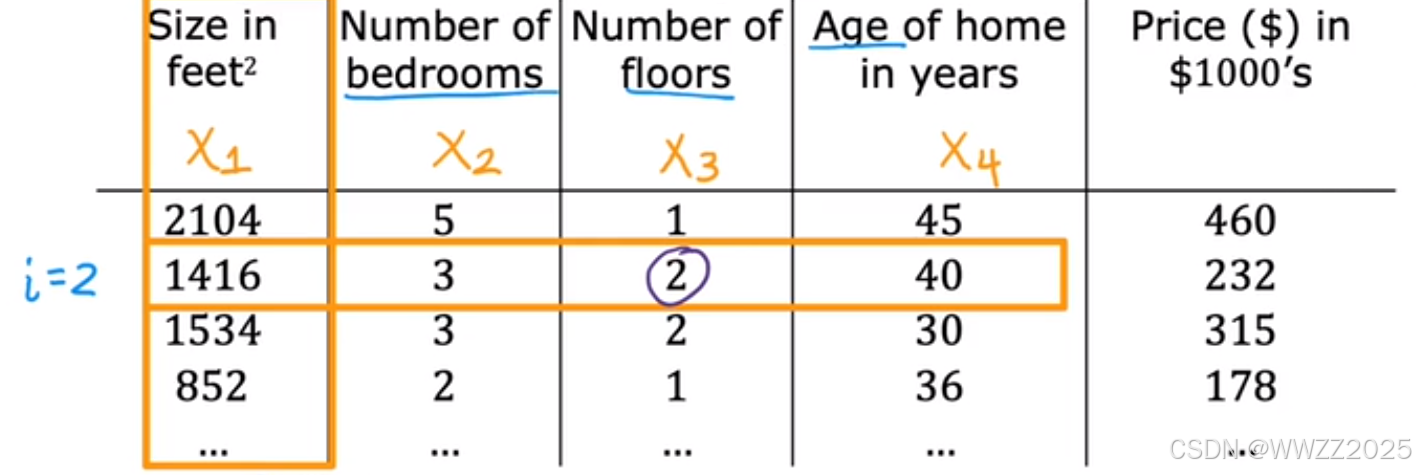
输出:

复制代码
Iteration    0: Cost  2529.46   
Iteration  100: Cost   695.99   
Iteration  200: Cost   694.92   
Iteration  300: Cost   693.86   
Iteration  400: Cost   692.81   
Iteration  500: Cost   691.77   
Iteration  600: Cost   690.73   
Iteration  700: Cost   689.71   
Iteration  800: Cost   688.70   
Iteration  900: Cost   687.69   
b,w found by gradient descent: -0.00,[ 0.2   0.   -0.01 -0.07] 
prediction: 426.19, target value: 460
prediction: 286.17, target value: 232
prediction: 171.47, target value: 178

4 正规方程(Normal equation)求解代价函数

采用正规方程可以直接求解w,b,无需使用梯度下降法迭代。

4.1 定义

仅用于线性回归,用于直接求解w,b而不需迭代。

4.2 缺点

(1)无法推广到其他算法;

(2)特征量n很大(>10000)运算很慢

相关推荐
deephub3 小时前
深入BERT内核:用数学解密掩码语言模型的工作原理
人工智能·深度学习·语言模型·bert·transformer
PKNLP3 小时前
BERT系列模型
人工智能·深度学习·bert
兰亭妙微4 小时前
ui设计公司审美积累 | 金融人工智能与用户体验 用户界面仪表盘设计
人工智能·金融·ux
东方佑4 小时前
从字符串中提取重复子串的Python算法解析
windows·python·算法
西阳未落4 小时前
LeetCode——二分(进阶)
算法·leetcode·职场和发展
通信小呆呆4 小时前
以矩阵视角统一理解:外积、Kronecker 积与 Khatri–Rao 积(含MATLAB可视化)
线性代数·算法·matlab·矩阵·信号处理
AKAMAI4 小时前
安全风暴的绝地反击 :从告警地狱到智能防护
运维·人工智能·云计算
岁月宁静5 小时前
深度定制:在 Vue 3.5 应用中集成流式 AI 写作助手的实践
前端·vue.js·人工智能
galaxylove5 小时前
Gartner发布数据安全态势管理市场指南:将功能扩展到AI的特定数据安全保护是DSPM发展方向
大数据·人工智能