TensorFlow深度学习实战——链路预测

TensorFlow深度学习实战------链路预测

- [0. 前言](#0. 前言)
- [1. 链路预测任务](#1. 链路预测任务)
- [2. 数据导入与处理](#2. 数据导入与处理)
- [3. 构建链路预测模型](#3. 构建链路预测模型)
- [4. 模型训练与评估](#4. 模型训练与评估)
- 相关链接

0. 前言

链路预测是一种边分类问题，任务是预测图中两个给定节点之间是否存在边。许多应用，如社交推荐、知识图谱补全等，都可以形式化为链路预测，即预测一对节点之间是否存在边。在本节中，我们将预测在引文网络中，两个论文之间是否存在引用关系(包括引用和被引用)。

1. 链路预测任务

链接预测 (Link prediction，也称链路预测)是图学习中的常见任务之一，用于预测两个节点之间是否存在链接的问题。链接预测是社交网络和推荐系统的核心，例如，在社交网络中，链接预测可以用于发现潜在的朋友关系、推荐共同的兴趣爱好，或者预测用户之间的互动行为。直观地说，如果存在链接的可能性很高，就更有可能与这些人建立联系，这种可能性正是链接预测试图预测的内容。

通常的方法是将图中的所有边视为正样本，从中采样一些不存在的边作为负样本，然后使用这些正负样本训练二分类(边是否存在)链路预测模型。

2. 数据导入与处理

首先导入所需的库：

python 复制代码

import dgl
import dgl.data
import dgl.function as fn
import tensorflow as tf
import itertools
import numpy as np
import scipy.sparse as sp
from dgl.nn import SAGEConv
from sklearn.metrics import roc_auc_score

重用在节点分类一节使用的 CORA 引文数据集：

python 复制代码

"""Loading Graph and Features"""
dataset = dgl.data.CoraGraphDataset()
g = dataset[0]

准备数据。为了训练链路预测模型，需要一组正样本和一组负样本。正样本是 CORA 引文图中已经存在的 10,556 条边，而负边是从图的其余部分中随机采样的 10,556 对没有连接边的节点对。此外，还需要将正样本和负样本拆分为训练集、验证集和测试集：

python 复制代码

"""Prepare training and test sets"""
# Split edge set for training and testing
u, v = g.edges()

# positive edges
eids = np.arange(g.number_of_edges())
eids = np.random.permutation(eids)

test_size = int(len(eids) * 0.2)
val_size = int((len(eids) - test_size) * 0.1)
train_size = g.number_of_edges() - test_size - val_size

u = u.numpy()
v = v.numpy()

test_pos_u = u[eids[0:test_size]]
test_pos_v = v[eids[0:test_size]]
val_pos_u = u[eids[test_size:test_size + val_size]]
val_pos_v = v[eids[test_size:test_size + val_size]]
train_pos_u = u[eids[test_size + val_size:]]
train_pos_v = v[eids[test_size + val_size:]]

print(train_pos_u.shape, train_pos_v.shape, 
      val_pos_u.shape, val_pos_v.shape,
      test_pos_u.shape, test_pos_v.shape)

# negative edges
adj = sp.coo_matrix((np.ones(len(u)), (u, v)))
adj_neg = 1 - adj.todense() - np.eye(g.number_of_nodes())
neg_u, neg_v = np.where(adj_neg != 0)

neg_eids = np.random.choice(len(neg_u), g.number_of_edges())
test_neg_u = neg_u[neg_eids[:test_size]]
test_neg_v = neg_v[neg_eids[:test_size]]
val_neg_u = neg_u[neg_eids[test_size:test_size + val_size]]
val_neg_v = neg_v[neg_eids[test_size:test_size + val_size]]
train_neg_u = neg_u[neg_eids[test_size + val_size:]]
train_neg_v = neg_v[neg_eids[test_size + val_size:]]

print(train_neg_u.shape, train_neg_v.shape, 
      val_neg_u.shape, val_neg_v.shape,
      test_neg_u.shape, test_neg_v.shape)

# remove edges from training graph
test_edges = eids[:test_size]
val_edges = eids[test_size:test_size + val_size]
train_edges = eids[test_size + val_size:]
train_g = dgl.remove_edges(g, np.concatenate([test_edges, val_edges]))

3. 构建链路预测模型

构建图神经网络 (Graph Neural Network, GNN)，使用两个 GraphSAGE 层计算节点表示，每层通过平均其邻居的信息来计算节点表示：

python 复制代码

"""Define a GraphSAGE Model"""
class LinkPredictor(tf.keras.Model):
    def __init__(self, g, in_feats, h_feats):
        super(LinkPredictor, self).__init__()
        self.g = g
        self.conv1 = SAGEConv(in_feats, h_feats, 'mean')
        self.relu1 = tf.keras.layers.Activation(tf.nn.relu)
        self.conv2 = SAGEConv(h_feats, h_feats, 'mean')

    def call(self, in_feat):
        h = self.conv1(self.g, in_feat)
        h = self.relu1(h)
        h = self.conv2(self.g, h)
        return h

链路预测需要计算节点对的表示，DGL 推荐将节点对视为另一个图，因为可以将一对节点定义为一条边。对于链路预测，有一个包含所有正样本边的正样本图和一个包含所有负样本边的负样本图，正样本图和负样本图都包含与原始图相同的节点集：

python 复制代码

train_pos_g = dgl.graph((train_pos_u, train_pos_v), num_nodes=g.number_of_nodes())
train_neg_g = dgl.graph((train_neg_u, train_neg_v), num_nodes=g.number_of_nodes())

val_pos_g = dgl.graph((val_pos_u, val_pos_v), num_nodes=g.number_of_nodes())
val_neg_g = dgl.graph((val_neg_u, val_neg_v), num_nodes=g.number_of_nodes())

test_pos_g = dgl.graph((test_pos_u, test_pos_v), num_nodes=g.number_of_nodes())
test_neg_g = dgl.graph((test_neg_u, test_neg_v), num_nodes=g.number_of_nodes())

接下来，定义一个预测器类，使用 LinkPredictor 类中的节点表示集，并使用 DGLGraph.apply_edges 方法计算边特征分数，这些分数是源节点特征和目标节点特征的点积：

python 复制代码

class DotProductPredictor(tf.keras.Model):
    def call(self, g, h):
        with g.local_scope():
            g.ndata['h'] = h
            # Compute a new edge feature named 'score' by a dot-product between the
            # source node feature 'h' and destination node feature 'h'.
            g.apply_edges(fn.u_dot_v('h', 'h', 'score'))
            # u_dot_v returns a 1-element vector for each edge so you need to squeeze it.
            return g.edata['score'][:, 0]

此外，也可以构建其它类型的自定义预测器，例如具有两个全连接层的多层感知机，apply_edges 方法描述了边特征分数的计算方式：

python 复制代码

class MLPPredictor(tf.keras.Model):
    def __init__(self, h_feats):
        super().__init__()
        self.W1 = tf.keras.layers.Dense(h_feats, activation=tf.nn.relu)
        self.W2 = tf.keras.layers.Dense(1)

    def apply_edges(self, edges):
        """
        Computes a scalar score for each edge of the given graph.

        Parameters
        ----------
        edges :
        Has three members ``src``, ``dst`` and ``data``, each of
        which is a dictionary representing the features of the
        source nodes, the destination nodes, and the edges
        themselves.

        Returns
        -------
        dict
        A dictionary of new edge features.
        """
        h = tf.concat([edges.src["h"], edges.dst["h"]], axis=1)
        return {"score": self.W2(self.W1(h))[:, 0]}

    def call(self, g, h):
        with g.local_scope():
            g.ndata['h'] = h
            g.apply_edges(self.apply_edges)
            return g.edata['score']

实例化 LinkPredictor 模型，使用 Adam 优化器，损失函数为 BinaryCrossEntropy。在本节中，使用的预测头是 DotProductPredictor，但也可以替换为 MLPPredictor，pred 变量替换为 MLPPredictor 对象，而非 DotProductPredictor 对象：

python 复制代码

"""Training Loop (DotPredictor)"""
HIDDEN_SIZE = 16
LEARNING_RATE = 1e-2
NUM_EPOCHS = 100

# ----------- 3. set up loss and optimizer -------------- #
model = LinkPredictor(train_g, train_g.ndata['feat'].shape[1], HIDDEN_SIZE)
optimizer = tf.keras.optimizers.Adam(learning_rate=LEARNING_RATE)
loss_fcn = tf.keras.losses.BinaryCrossentropy(from_logits=True)

pred = DotProductPredictor()

4. 模型训练与评估

定义辅助函数用于训练循环。compute_loss() 函数计算从正样本图和负样本图中返回的分数之间的损失，compute_acc() 函数计算两个分数的曲线下面积 (Area Under the Curve, AUC)，AUC 是评估二分类模型的常用指标：

python 复制代码

def compute_loss(pos_score, neg_score):
    scores = tf.concat([pos_score, neg_score], axis=0)
    labels = tf.concat([
        tf.ones(pos_score.shape[0]), 
        tf.zeros(neg_score.shape[0])
    ], axis=0)
    return loss_fcn(labels, scores)


def compute_auc(pos_score, neg_score):
    scores = tf.concat([pos_score, neg_score], axis=0).numpy()
    labels = tf.concat([
        tf.ones(pos_score.shape[0]), 
        tf.zeros(neg_score.shape[0])
    ], axis=0).numpy()
    return roc_auc_score(labels, scores)

训练 LinkPredictor GNN 100 个 epoch：

python 复制代码

# ----------- 4. training -------------------------------- #
for epoch in range(NUM_EPOCHS):
    in_feat = train_g.ndata["feat"]
    with tf.GradientTape() as tape:
        h = model(in_feat)
        pos_score = pred(train_pos_g, h)
        neg_score = pred(train_neg_g, h)
        loss = compute_loss(pos_score, neg_score)
        grads = tape.gradient(loss, model.trainable_weights)
        optimizer.apply_gradients(zip(grads, model.trainable_weights))

    val_pos_score = pred(val_pos_g, h)
    val_neg_score = pred(val_neg_g, h)
    val_auc = compute_auc(val_pos_score, val_neg_score)

    if epoch % 5 == 0:
        print("Epoch {:3d} | train_loss: {:.3f}, val_auc: {:.3f}".format(
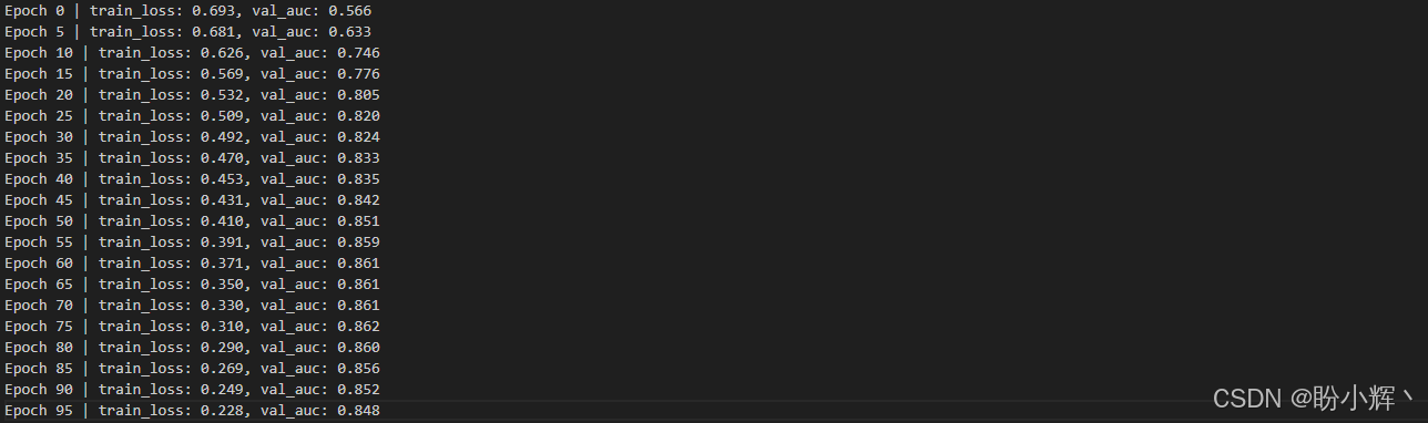
            epoch, loss, val_auc))

训练过程输出结果如下：

在测试集上评估训练后的模型：

python 复制代码

# ----------- 5. check results ------------------------ #
pos_score = tf.stop_gradient(pred(test_pos_g, h))
neg_score = tf.stop_gradient(pred(test_neg_g, h))
print('Test AUC', compute_auc(pos_score, neg_score))

LinkPredictor GNN 的测试 AUC如下：

python 复制代码

Test AUC 0.8266960571287392

可以看到，链接预测器可以准确预测测试集中 82% 的真实链接。

TensorFlow深度学习实战——链路预测

TensorFlow深度学习实战------链路预测

0. 前言

1. 链路预测任务

2. 数据导入与处理

3. 构建链路预测模型

4. 模型训练与评估

相关链接