mul 与 reduce_sum 的优化实例

一、基础介绍

什么是 mul 与 reduce_sum？

mul 通常指元素级乘法（Element-wise Multiplication），它将两个形状相同的张量中对应位置的元素相乘，返回一个与原张量形状相同的新张量。

reduce_sum 是一种规约操作（Reduction Operation），它沿指定维度对张量的元素求和，从而 "压缩" 或 "减少" 张量的维度。如果不指定维度，则对所有元素求和，返回一个标量。

二、baseline 结构

onnx 可视化图如下：

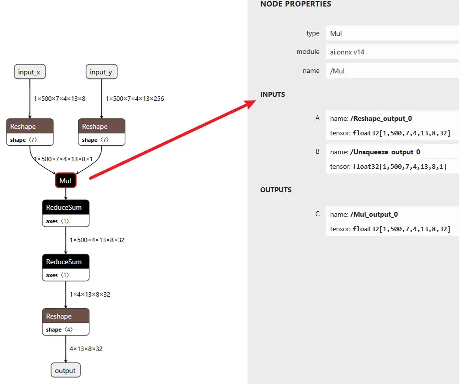
对应代码如下：

Plain 复制代码

class CustomNet(nn.Module):
    def __init__(self):
        super(CustomNet, self).__init__()

    def forward(self, a, b):
        # a: shape (1, 500, 7, 4, 13, 8)
        # b: shape (1, 500, 7, 4, 13, 256)
        # Step 1: Unsqueeze a -> (1, 500, 7, 4, 13, 8, 1)
        a = a.unsqueeze(-1)
        # Step 2: Reshape b -> (1, 500, 7, 4, 13, 8, 32)
        b = b.view(1, 500, 7, 4, 13, 8, 32)
        # Step 3: Mul (broadcast over last dim)
        out = a * b  # shape: (1, 500, 7, 4, 13, 8, 32)
        # # Step 4: ReduceSum over dim=2 (index 2 = 7 dim)
        out = out.sum(dim=2)  # shape: (1, 500, 4, 13, 8, 32)
        # # Step 5: ReduceSum over dim=1 (500 dim)
        out = out.sum(dim=1)  # shape: (1, 4, 13, 8, 32)
        # Step 6: Reshape to final output
        out = out.view(-1, 13, 8, 32)  # 可根据需要调整最终输出 shape
        return out
        
a = torch.randn(1, 500, 7, 4, 13, 8)
b = torch.randn(1, 500, 7, 4, 13, 256)
model = CustomNet()
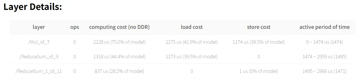
output = model(a, b)

在征程 6M 上进行简单的模型编译与性能预估：

Plain 复制代码

hb_compile -m mymodel.onnx --march nash-m --fast-perf

根据产出物得到预估 latency：2.97 ms

这个结构如何进行优化呢？

三、合并 reduce_sum

Plain 复制代码

# Step 4: ReduceSum over dim=2 (index 2 = 7 dim)
out = out.sum(dim=2)  # shape: (1, 500, 4, 13, 8, 32)

# Step 5: ReduceSum over dim=1 (500 dim)
out = out.sum(dim=1)  # shape: (1, 4, 13, 8, 32)

这两个 reducesum 能合并成一个，使用 dim=（1， 2）（即同时对 dim=1 和 dim=2 做 sum），前提是这两个维度的求和没有先后顺序依赖（即两个维度是独立的）

Plain 复制代码

out = out.sum(dim=(1, 2))  # 一次性对 dim=1 和 dim=2 求和

PyTorch 中。sum（dim=（1， 2））会按照给出的维度一次性执行 sum 操作，等价于逐个做 dim=2 然后 dim=1，因为 sum 是可交换的操作，最终结果形状完全相同。

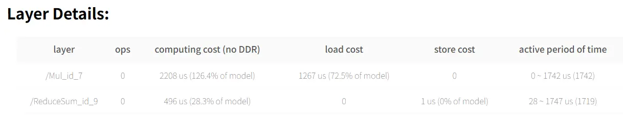
优化后结构如下，可以看到确实少了一个 reducesum：

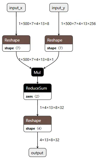
预估 latency: 1.75 ms

四、mul+reducesum 变成 conv

假设有两个张量：

a.shape = (B, C, H, W)
b.shape = (B, C, H, W)

常见操作是：

Plain 复制代码

out = (a * b).sum(dim=[2, 3])  # 在 H 和 W 上求和，输出 shape: (B, C)

# ----------细节---------------
import torch
import torch.nn as nn
a = torch.randn(1, 3, 8, 4) # 多维时，a的最后一维若与b不同，则只能是1，否则不能进行广播
b = torch.randn(1, 3, 8, 4)
c = a * b               # c的shape：torch.Size([1, 3, 8, 4])
d = c.sum(dim=[2,3])    # d的shape：torch.Size([1, 3])

注意：torch 中 a * b 是逐元素相乘（mul），而不是矩阵乘法（matmul），形状不匹配时会触发广播（复制对应列 or 行）

通过深度卷积（depthwise convolution）可以近似实现 Mul + ReduceSum 操作，等价的 Conv2d 实现方式，可以用 groups=B*C 的 conv2d 来实现上述操作：

Plain 复制代码

import torch
import torch.nn.functional as F

def conv_approx_mul_reducesum(a, b):
    B, C, H, W = a.shape

    # 把 b 变成卷积核，作为每个通道的 filter
    kernel = b.reshape(B * C, 1, H, W)

    # 输入 reshape 成 (1, B*C, H, W)
    input_ = a.reshape(1, B * C, H, W)

    # 深度卷积实现 mul+sum，输出 shape: (1, B*C, 1, 1)
    output = F.conv2d(input_, kernel, groups=B * C)

    # reshape 回 (B, C)
    return output.reshape(B, C)

conv2d 的过程是：

对每个通道进行乘法（卷积）
然后在 kernel 区域内求和

所以 F.conv2d（a， b， groups=B*C）本质就是：对 a 和 b 逐元素相乘再求和 = Mul + ReduceSum

一致性验证：

Plain 复制代码

import torch
import torch.nn as nn
import torch.nn.functional as F

a = torch.randn(1, 3, 8, 4) # 多维时，a的最后一维若与b不同，则只能是1，否则不能进行广播
b = torch.randn(1, 3, 8, 4)
c = a * b               # c的shape：torch.Size([1, 3, 8, 4])
d = c.sum(dim=[2,3])    # d的shape：torch.Size([1, 3])
print(d)


def F_conv2d_approx_mul_reducesum(a, b):
    B, C, H, W = a.shape

    # 把 b 变成卷积核，作为每个通道的 filter
    kernel = b.reshape(B * C, 1, H, W)

    # 输入 reshape 成 (1, B*C, H, W)
    input_ = a.reshape(1, B * C, H, W)

    # 深度卷积实现 mul+sum，输出 shape: (1, B*C, 1, 1)
    output = F.conv2d(input_, kernel, groups=B * C)

    # reshape 回 (B, C)
    return output.reshape(B, C)
print(F_conv2d_approx_mul_reducesum(a,b))


def nn_conv2d_approx_mul_reducesum(a, b):
    B, C, H, W = a.shape

    # 把 b 变成卷积核，作为每个通道的 filter
    kernel = b.reshape(B * C, 1, H, W)

    # 输入 reshape 成 (1, B*C, H, W)
    input_ = a.reshape(1, B * C, H, W)

    # 假设已有输入input_和卷积核kernel
    # kernel形状: (输出通道数, 输入通道数//groups, 核高, 核宽)
    # 例如：groups=B*C时，输入通道数需为groups的倍数
    out_channels = kernel.size(0)
    in_channels = kernel.size(1) * (B * C)  # 输入通道数 = 每组通道数 * groups
    kernel_size = (kernel.size(2), kernel.size(3))
    # 创建nn.Conv2d模块
    conv_layer = nn.Conv2d(
        in_channels=in_channels,
        out_channels=out_channels,
        kernel_size=kernel_size,
        groups=B * C,
        bias=False  # 若F.conv2d未用偏置
    )
    # 将预定义的kernel赋值给conv_layer的权重
    conv_layer.weight.data = kernel  # 注意：需确保kernel形状与nn.Conv2d的weight格式一致

    # 深度卷积实现 mul+sum，输出 shape: (1, B*C, 1, 1)
    output = conv_layer(input_)

    # reshape 回 (B, C)
    return output.reshape(B, C)
print(nn_conv2d_approx_mul_reducesum(a,b))

输出：

Plain 复制代码

tensor([[-0.3991,  0.2382, -8.5925]])
tensor([[-0.3991,  0.2382, -8.5925]])
tensor([[-0.3991,  0.2382, -8.5925]], grad_fn=<ViewBackward0>)

可以看到，结果确实一样。

真正部署时，不太建议这么做，因为小尺寸没必要（快不了多少），大尺寸硬件不支持。