本文通过生活化的比喻和直观的视觉化讲解,带你一步步理解神经网络如何通过"前向猜测"和"反向追责"实现学习,无需深厚数学基础也能掌握这一AI核心原理。
一、引言:当我们摔倒时,大脑在做什么?
还记得第一次学骑自行车的场景吗?歪歪扭扭、摔倒、爬起来、调整姿势、再尝试......直到最终能够平稳骑行。
这个尝试→犯错→调整→再尝试 的过程,正是我们人类学习的本质。而今天要介绍的BP神经网络,就是计算机科学家模仿这种"试错学习"机制创造的人工智能模型。
如果把神经网络比作一个学生,那么反向传播就是它的"后悔药"------让AI能够从错误中学习,变得越来越聪明。
二、第一部分:前向传播------大脑的第一次猜测
1.巧克力工厂生产线:理解神经网络结构
想象一个巧克力工厂的生产线:
-
输入层:原料准备区(可可豆、糖、牛奶)
-
隐藏层:加工车间(研磨、混合、调温)
-
输出层:包装检验区(成品巧克力)
-
权重(w):管道粗细(决定原料流量)
-
偏置(b):调味秘方(基础风味)
前向传播过程演示:
-
可可豆(输入x₁=1)通过粗管道(w₁=0.8)进入隐藏层第一车间
-
糖(输入x₂=1)通过细管道(w₂=0.3)进入同一车间
-
车间对来料进行加工:
0.8*1 + 0.3*1 + 秘方(0.1) = 1.2 -
这个值经过"调味机"(激活函数Sigmoid):
1/(1+e^(-1.2)) ≈ 0.77 -
0.77作为半成品流向下一车间,最终产出"巧克力"(预测输出)
2.第一次品尝:发现误差
工厂生产出了巧克力,我们品尝后打分:
-
预测值:甜度0.85(网络的输出)
-
真实值:甜度0.90(实际应该达到的标准)
-
误差 :
0.85 - 0.90 = -0.05(不够甜)
关键问题:这个误差是谁的责任?是可可豆质量不好?糖放少了?还是管道太细了?
三、第二部分:反向传播------AI的"责任追溯"与改进
1.工厂质量事故调查会
输出层(总经理)很生气:"巧克力甜度不够!误差-0.05!"
追责流程开始:
-
包装车间:"我们只负责包装,但加工车间给的半成品就不够甜!"
-
加工车间:"我们按照配方做的,但原料来的时候就不够甜!"
-
原料采购:"我们按照规定的管道粗细买的原料!"
核心思想 :误差按照"贡献比例"反向分配,形成一条完整的责任链。
2.数学思想的直观理解(不涉及复杂公式)
每个"车间"(神经元)对最终误差的责任 = 当前车间影响力 × 下一车间的责任
其中:
-
影响力 = 管道粗细(权重)× 当前车间的敏感度(导数)
-
敏感度:衡量该车间输出对输入变化的反应程度
3.梯度下降:下山找最优解
我们的目标是找到误差最低点(最美味的巧克力配方)。现在站在半山腰(当前参数配置),需要找到下山最快的方向。
学习率 :下山时的步长
-
步长太大:可能错过最佳点,在山谷两侧震荡
-
步长太小:下山速度太慢,训练效率低下
-
策略:小步快跑(适中的学习率)
权重更新演示
调查清楚了责任分配:
- 可可豆管道责任小,糖管道责任大
调整管道粗细:
老管道: w₁=0.8(可可豆), w₂=0.3(糖)
调整后:w₁=0.82(+0.02), w₂=0.25(-0.05)
一句话总结反向传播 :责任追溯 + 梯度下山
四、第三部分:完整学习流程------以"学认数字"为例
1.手写数字识别实战演示
以经典的MNIST手写数字识别为例:
-
网络结构:
-
输入层:784个神经元(28×28像素)
-
隐藏层:16个神经元
-
输出层:10个神经元(对应数字0-9)
-
-
学习过程:
-
前向传播:输入"8"的图片 → 网络猜测是"6"(错了!)
-
误差计算:对于"6"的输出应该是0,实际是0.9;对于"8"应该是1,实际只有0.1
-
反向传播:误差从输出层反向流回,告诉网络"把8认成6是大错特错"
-
权重调整:降低"6"神经元的敏感性,增强"8"神经元的权重
-
再次尝试:同样的"8"图片 → 输出"8"的概率提高到0.7!
-
顿悟时刻:看!网络通过一次反思,就变得更聪明了!
2.互动游戏:体验神经网络的学习
想象8个同学组成一个微型神经网络:
- 3个输入层同学 → 4个隐藏层同学 → 1个输出层同学
游戏规则:
-
前向传播阶段:老师给出输入1,0,1,每个"神经元"按自己的权重计算并传递
-
预测阶段:输出层同学说出预测值(如0.6)
-
真相揭晓:老师公布真实值(0.9)
-
反向传播阶段:输出层计算误差,告诉前一层"你该负多少责"
-
调整阶段:每个同学根据"责任"调整自己的"权重卡片"
通过这个游戏,你能亲身感受误差如何从后往前传,以及每个"神经元"如何"反思改进"。
五、第四部分:为什么有效?------从量变到质变的智慧
1.一次错误 vs 千万次训练
关键洞察:单次调整可能不明显,但成千上万次调整后,量变引起质变。
就像学生做1000道数学题:
-
每错一题就搞懂为什么错
-
1000题后,就成了学霸!
训练相关术语:
-
一个样本 = 一道题
-
一个epoch = 刷一遍题库
-
批量训练 = 做完一批题再统一订正
2.深度网络的威力:为什么需要多层?
浅层网络局限:只能学习简单模式(如用直线分割数据)
深层网络优势:可以学习复杂、抽象的模式
以识别"猫"的深度网络为例:
第一层:识别边缘(直线、曲线)
第二层:识别形状(圆形、三角形)
第三层:识别部件(耳朵、胡须、眼睛)
第四层:识别整体(猫脸)BP的核心价值:正是反向传播,让这么深层的网络能够"层层追责",最终调整所有参数,学习到这种层次化的特征表示。
六、第五部分:BP神经网络学习法总结
1.完整学习流程比喻
BP神经网络就像一个有自省能力的学生:
-
前向传播:做一道题,给出答案
-
得到批改:老师打叉,知道错了多少
-
反向传播:从最后一步开始,一步步往前反思
-
梯度下降:找到改进方向,调整解题思路
-
再次尝试:类似题目,正确率提高!
核心公式一览(思想重于形式)
# 前向传播(做预测)
预测值 = sigmoid(权重 * 输入 + 偏置)

# 计算误差
误差 = 预测值 - 真实值

# 反向传播(链式法则)
输出层误差 = 误差 * sigmoid的敏感度
隐藏层误差 = 输出层误差 * 权重 * 上一层的敏感度

# 权重更新(梯度下降)
新权重 = 旧权重 - 学习率 * (误差对权重的导数)
重要提示 :公式背后的思想比公式本身更重要!
七、技术细节与代码实现
极简BP神经网络实现
python
import numpy as np

class SimpleNN:
    def __init__(self):
        # 随机初始化权重(就像随机猜测)
        self.w = np.random.randn(3, 1)  # 3个输入到1个输出的权重
        self.b = np.random.randn()      # 偏置

    def sigmoid(self, x):
        return 1 / (1 + np.exp(-x))

    def forward(self, x):
        # 前向传播:计算预测值
        z = np.dot(x, self.w) + self.b
        return self.sigmoid(z)

    def train_one_step(self, x, y_true, learning_rate=0.1):
        # 一次完整的训练:前向 + 反向 + 更新
        # 1. 前向传播
        y_pred = self.forward(x)

        # 2. 计算误差
        error = y_pred - y_true

        # 3. 反向传播(简化版链式法则)
        w_grad = x * error * y_pred * (1 - y_pred)
        b_grad = error * y_pred * (1 - y_pred)

        # 4. 梯度下降更新权重
        self.w -= learning_rate * w_grad.reshape(-1, 1)
        self.b -= learning_rate * b_grad

        return error

# 创建网络实例
nn = SimpleNN()

# 训练数据:学习逻辑与门(AND)
X = np.array([[0,0,1], [0,1,1], [1,0,1], [1,1,1]])  # 第三列是偏置的固定输入1
y = np.array([0, 0, 0, 1])  # AND门的结果

print("训练前预测:")
for i in range(4):
    print(f"输入{X[i,:-1]} -> 预测{nn.forward(X[i]):.3f} (应该是{y[i]})")

print("\n开始训练...")
for epoch in range(100):
    for i in range(4):
        nn.train_one_step(X[i], y[i])

print("\n训练后预测:")
for i in range(4):
    print(f"输入{X[i,:-1]} -> 预测{nn.forward(X[i]):.3f} (应该是{y[i]})")
八、常见问题解答
1.链式求导太难理解
今天我们不需要会求导,只需要理解"责任追溯"的思想。就像追查事故责任,你不需要懂所有法律条文,只需要知道谁该负责。
2.为什么叫反向传播
因为误差是从输出层开始,一层层往回(反向)传递责任,调整前面的参数。
3.学习率太大或太小会怎样
- 学习率太大(步子太大)会在山谷两边跳来跳去,无法收敛;
- 学习率太小(步子太小)则学习速度太慢。需要找到合适的小步快跑节奏。
4.为什么需要激活函数
没有激活函数,无论多少层网络都等价于单层线性网络,无法学习复杂模式。
激活函数引入了非线性,让网络能够拟合任意复杂函数。
九、现实应用与展望
BP神经网络及其变体已广泛应用于:
-
语音助手:Siri/Alexa如何听懂你的话
-
自动驾驶:汽车如何识别行人和交通标志
-
推荐系统:抖音/淘宝如何知道你喜欢什么
-
医疗诊断:辅助医生识别医学影像
十、项目实战:基于BP神经网络的医学影像辅助诊断系统实现
1.项目概述
下面使用BP神经网络实现一个医疗影像辅助诊断系统,以识别肺部X光片是否显示肺炎症状为例。我们将从数据准备、网络设计、训练优化到结果分析,完整展示BP神经网络在医疗诊断中的应用。
**2.**数据准备与预处理
我们将使用公开的胸部X光影像数据集(COVID-19 Radiography Database),该数据集包含正常和肺炎患者的X光影像。
python
import numpy as np
import pandas as pd
import matplotlib.pyplot as plt
import seaborn as sns
from sklearn.model_selection import train_test_split
from sklearn.preprocessing import LabelEncoder
import cv2
import os
import warnings
warnings.filterwarnings('ignore')

# 设置随机种子确保可重复性
np.random.seed(42)

# 数据路径(实际使用时需要修改为真实路径)
# 这里我们使用模拟数据生成来演示流程
class MedicalImageDataGenerator:
    def __init__(self, image_size=(64, 64)):
        self.image_size = image_size
        self.classes = ['normal', 'pneumonia']

    def generate_synthetic_dataset(self, n_samples=1000):
        """
        生成模拟的医学影像数据集
        在实际应用中,应该使用真实数据替换此函数
        """
        print("生成模拟医学影像数据集...")

        # 创建模拟数据
        X = []
        y = []

        for i in range(n_samples):
            # 随机决定类别(70%正常,30%肺炎)
            if np.random.rand() < 0.7:
                label = 0  # 正常
                # 正常肺部X光特征:较清晰的纹理,较暗的背景
                img = self._generate_normal_lung_image()
            else:
                label = 1  # 肺炎
                # 肺炎肺部X光特征:模糊的纹理,局部高亮区域
                img = self._generate_pneumonia_lung_image()

            X.append(img.flatten())  # 将图像展平为一维向量
            y.append(label)

        X = np.array(X)
        y = np.array(y)

        print(f"数据集生成完成: {X.shape[0]}个样本, {X.shape[1]}个特征")
        print(f"类别分布: 正常={np.sum(y==0)}, 肺炎={np.sum(y==1)}")

        return X, y

    def _generate_normal_lung_image(self):
        """生成正常肺部X光模拟图像"""
        img = np.zeros(self.image_size)

        # 模拟肺部区域(两个较暗的椭圆形区域)
        h, w = self.image_size
        center_x1, center_y1 = w//3, h//2
        center_x2, center_y2 = 2*w//3, h//2

        # 生成两个肺叶
        for i in range(h):
            for j in range(w):
                # 左肺
                dist1 = np.sqrt((i-center_y1)**2 + (j-center_x1)**2)
                # 右肺
                dist2 = np.sqrt((i-center_y2)**2 + (j-center_x2)**2)

                if dist1 < h//4:
                    img[i, j] = 0.3 + 0.2 * np.random.rand()  # 肺部区域较暗
                elif dist2 < h//4:
                    img[i, j] = 0.3 + 0.2 * np.random.rand()  # 肺部区域较暗
                else:
                    img[i, j] = 0.7 + 0.3 * np.random.rand()  # 背景较亮

        # 添加一些正常纹理
        img += 0.1 * np.random.randn(*self.image_size)
        img = np.clip(img, 0, 1)

        return img

    def _generate_pneumonia_lung_image(self):
        """生成肺炎肺部X光模拟图像"""
        img = np.zeros(self.image_size)

        # 先创建正常肺部基础
        h, w = self.image_size
        center_x1, center_y1 = w//3, h//2
        center_x2, center_y2 = 2*w//3, h//2

        # 生成两个肺叶(基础)
        for i in range(h):
            for j in range(w):
                dist1 = np.sqrt((i-center_y1)**2 + (j-center_x1)**2)
                dist2 = np.sqrt((i-center_y2)**2 + (j-center_x2)**2)

                if dist1 < h//4 or dist2 < h//4:
                    img[i, j] = 0.4 + 0.3 * np.random.rand()  # 肺炎时肺部区域较亮
                else:
                    img[i, j] = 0.6 + 0.4 * np.random.rand()  # 背景

        # 添加肺炎特征:局部高亮区域(炎症)
        pneumonia_patches = np.random.randint(2, 5)  # 2-4个炎症区域
        for _ in range(pneumonia_patches):
            patch_x = np.random.randint(w//4, 3*w//4)
            patch_y = np.random.randint(h//4, 3*h//4)
            patch_size = np.random.randint(5, 15)

            for i in range(max(0, patch_y-patch_size), min(h, patch_y+patch_size)):
                for j in range(max(0, patch_x-patch_size), min(w, patch_x+patch_size)):
                    if np.sqrt((i-patch_y)**2 + (j-patch_x)**2) < patch_size:
                        img[i, j] = min(1.0, img[i, j] + 0.3)  # 增加亮度表示炎症

        # 添加纹理噪声
        img += 0.15 * np.random.randn(*self.image_size)
        img = np.clip(img, 0, 1)

        return img

    def visualize_samples(self, X, y, n_samples=4):
        """可视化样本"""
        fig, axes = plt.subplots(2, n_samples//2, figsize=(12, 6))
        axes = axes.flatten()

        indices = np.random.choice(len(X), n_samples, replace=False)

        for idx, ax in enumerate(axes):
            sample_idx = indices[idx]
            img = X[sample_idx].reshape(self.image_size)
            label = y[sample_idx]

            ax.imshow(img, cmap='gray')
            ax.set_title(f"样本 {sample_idx}: {'肺炎' if label==1 else '正常'}")
            ax.axis('off')

        plt.tight_layout()
        plt.show()

# 生成数据集
data_gen = MedicalImageDataGenerator(image_size=(64, 64))
X, y = data_gen.generate_synthetic_dataset(n_samples=1200)

# 可视化部分样本
print("\n样本可视化:")
data_gen.visualize_samples(X, y, n_samples=6)

# 数据集划分
X_train, X_test, y_train, y_test = train_test_split(
    X, y, test_size=0.2, random_state=42, stratify=y
)

X_train, X_val, y_train, y_val = train_test_split(
    X_train, y_train, test_size=0.125, random_state=42, stratify=y_train  # 0.125*0.8=0.1
)

print(f"\n数据集划分:")
print(f"训练集: {X_train.shape[0]} 个样本")
print(f"验证集: {X_val.shape[0]} 个样本")
print(f"测试集: {X_test.shape[0]} 个样本")这段代码是一个医学影像数据模拟生成与预处理的完整流程 。它通过定义一个专门的MedicalImageDataGenerator类,创建了一个虚拟的胸部X光图像数据集,用于肺炎检测任务的演示。该类能够生成两类模拟图像:正常的肺部X光图像显示为较暗的椭圆形区域,而肺炎病例的图像则在此基础上添加局部高亮区域来模拟炎症特征。整个系统生成了1200个64×64像素的样本,其中70%标记为正常,30%标记为肺炎,完美模拟了真实医学数据集中常见的类别不平衡问题。
在数据处理方面,代码采用了标准化的机器学习工作流程。生成的数据集被划分为训练集、验证集和测试集,比例分别为70%、10%和20%,并且使用分层抽样确保了每个子集中类别比例的一致性。同时,代码包含了可视化功能,能够随机展示样本图像及其标签,帮助用户直观理解数据特征。这种划分方式为后续构建和评估分类模型奠定了坚实的基础。
这段代码的核心价值在于教学与演示,它展示了一个完整的医学影像分析项目的前期数据准备阶段。尽管生成的是模拟数据,但它精确地模拟了真实医学图像的关键特征,并为真实场景中的数据加载和预处理提供了可参考的框架。在实际应用中,开发者只需替换数据生成部分为真实医学影像数据,即可快速迁移到实际的肺炎检测或其他医学影像分析任务中。
3. 数据标准化与增强
python
class DataPreprocessor:
    def __init__(self):
        self.mean = None
        self.std = None

    def fit_transform(self, X_train):
        """计算并应用标准化"""
        self.mean = np.mean(X_train, axis=0)
        self.std = np.std(X_train, axis=0)
        self.std[self.std == 0] = 1  # 避免除零

        X_train_normalized = (X_train - self.mean) / self.std
        return X_train_normalized

    def transform(self, X):
        """应用标准化"""
        if self.mean is None or self.std is None:
            raise ValueError("必须先使用fit_transform方法")
        return (X - self.mean) / self.std

    def apply_data_augmentation(self, X, y, augmentation_factor=2):
        """数据增强:增加训练数据多样性"""
        print(f"应用数据增强...")

        X_augmented = [X]
        y_augmented = [y]

        # 对训练数据进行简单增强
        for _ in range(augmentation_factor - 1):
            X_noisy = X + 0.05 * np.random.randn(*X.shape)  # 添加噪声
            X_noisy = np.clip(X_noisy, -3, 3)  # 限制在合理范围内

            X_augmented.append(X_noisy)
            y_augmented.append(y)

        X_augmented = np.vstack(X_augmented)
        y_augmented = np.hstack(y_augmented)

        # 打乱增强后的数据
        shuffle_idx = np.random.permutation(len(X_augmented))
        X_augmented = X_augmented[shuffle_idx]
        y_augmented = y_augmented[shuffle_idx]

        print(f"数据增强完成: {len(X_augmented)} 个样本")
        return X_augmented, y_augmented

# 数据预处理
preprocessor = DataPreprocessor()
X_train_normalized = preprocessor.fit_transform(X_train)
X_val_normalized = preprocessor.transform(X_val)
X_test_normalized = preprocessor.transform(X_test)

# 数据增强(仅对训练集)
X_train_augmented, y_train_augmented = preprocessor.apply_data_augmentation(
    X_train_normalized, y_train, augmentation_factor=2
)

print(f"\n增强后训练集: {X_train_augmented.shape[0]} 个样本")
这段代码定义了一个名为 DataPreprocessor 的类,专门用于医学影像数据的标准化预处理和数据增强。该类包含三个核心方法:fit_transform 方法用于计算训练数据的均值和标准差并完成标准化;transform 方法利用已计算的统计量对新数据进行同样的标准化处理;apply_data_augmentation 方法则通过向训练数据添加可控的高斯噪声来生成增强样本,从而提高数据的多样性并打乱顺序,为模型训练提供更丰富的学习材料。
代码执行部分创建了 DataPreprocessor 的实例,首先对整个数据集(训练集、验证集、测试集)进行了标准化处理,确保所有数据具有相同的尺度。然后,它仅对标准化后的训练数据应用了数据增强技术,将训练样本数量扩展了一倍(通过 augmentation_factor=2 参数控制),从而在不改变数据分布本质的前提下,有效增加了训练集的规模和多样性,为后续训练鲁棒的机器学习模型奠定了重要基础。
这段代码的核心价值在于构建了一个完整且可复用的数据预处理管道,它遵循了机器学习中的最佳实践:基于训练集计算归一化参数并应用于所有数据集,仅对训练数据进行增强以避免数据泄漏。这样的设计不仅提升了模型训练的稳定性和效率,还通过数据增强策略缓解了医学影像数据通常面临的样本量有限问题,有助于改善模型的泛化能力和最终性能表现。
4.BP神经网络设计与实现
4.1 神经网络核心类
python
class BPNeuralNetwork:
    """
    用于医疗影像诊断的BP神经网络
    架构:输入层 → 隐藏层1 → 隐藏层2 → 输出层
    """
    def __init__(self, input_size, hidden1_size=128, hidden2_size=64, output_size=1,
                 learning_rate=0.01, activation='relu', dropout_rate=0.3):
        """
        初始化神经网络

        参数:
        - input_size: 输入特征维度
        - hidden1_size: 第一隐藏层神经元数量
        - hidden2_size: 第二隐藏层神经元数量
        - output_size: 输出层神经元数量(二分类为1)
        - learning_rate: 学习率
        - activation: 激活函数类型 ('sigmoid', 'relu', 'tanh')
        - dropout_rate: Dropout比例(防止过拟合)
        """
        # 网络参数
        self.input_size = input_size
        self.hidden1_size = hidden1_size
        self.hidden2_size = hidden2_size
        self.output_size = output_size
        self.learning_rate = learning_rate
        self.activation_type = activation
        self.dropout_rate = dropout_rate

        # 初始化权重和偏置
        self._initialize_weights()

        # 训练历史记录
        self.train_loss_history = []
        self.val_loss_history = []
        self.train_acc_history = []
        self.val_acc_history = []

        print(f"初始化神经网络: {input_size}→{hidden1_size}→{hidden2_size}→{output_size}")
        print(f"激活函数: {activation}, 学习率: {learning_rate}, Dropout率: {dropout_rate}")

    def _initialize_weights(self):
        """使用Xavier/Glorot初始化权重"""
        # 第一隐藏层权重
        limit1 = np.sqrt(6 / (self.input_size + self.hidden1_size))
        self.W1 = np.random.uniform(-limit1, limit1, (self.input_size, self.hidden1_size))
        self.b1 = np.zeros((1, self.hidden1_size))

        # 第二隐藏层权重
        limit2 = np.sqrt(6 / (self.hidden1_size + self.hidden2_size))
        self.W2 = np.random.uniform(-limit2, limit2, (self.hidden1_size, self.hidden2_size))
        self.b2 = np.zeros((1, self.hidden2_size))

        # 输出层权重
        limit3 = np.sqrt(6 / (self.hidden2_size + self.output_size))
        self.W3 = np.random.uniform(-limit3, limit3, (self.hidden2_size, self.output_size))
        self.b3 = np.zeros((1, self.output_size))

        # 创建动量项(用于动量梯度下降)
        self.momentum_W1 = np.zeros_like(self.W1)
        self.momentum_b1 = np.zeros_like(self.b1)
        self.momentum_W2 = np.zeros_like(self.W2)
        self.momentum_b2 = np.zeros_like(self.b2)
        self.momentum_W3 = np.zeros_like(self.W3)
        self.momentum_b3 = np.zeros_like(self.b3)

    def _activation(self, x, derivative=False):
        """激活函数"""
        if self.activation_type == 'sigmoid':
            if derivative:
                sig = 1 / (1 + np.exp(-x))
                return sig * (1 - sig)
            return 1 / (1 + np.exp(-x))

        elif self.activation_type == 'relu':
            if derivative:
                return (x > 0).astype(float)
            return np.maximum(0, x)

        elif self.activation_type == 'tanh':
            if derivative:
                return 1 - np.tanh(x)**2
            return np.tanh(x)

        else:
            raise ValueError(f"不支持的激活函数: {self.activation_type}")

    def _sigmoid(self, x, derivative=False):
        """Sigmoid函数(用于输出层)"""
        if derivative:
            sig = 1 / (1 + np.exp(-x))
            return sig * (1 - sig)
        return 1 / (1 + np.exp(-x))

    def _dropout(self, X, dropout_rate):
        """Dropout层(训练时使用)"""
        if dropout_rate > 0:
            mask = np.random.binomial(1, 1-dropout_rate, size=X.shape) / (1-dropout_rate)
            return X * mask
        return X

    def forward(self, X, training=True):
        """
        前向传播

        参数:
        - X: 输入数据 (batch_size, input_size)
        - training: 是否为训练模式(影响Dropout)

        返回:
        - output: 网络输出
        - cache: 缓存中间结果用于反向传播
        """
        # 输入层到第一隐藏层
        self.z1 = np.dot(X, self.W1) + self.b1
        self.a1 = self._activation(self.z1)

        # 应用Dropout(仅在训练时)
        if training:
            self.a1 = self._dropout(self.a1, self.dropout_rate)

        # 第一隐藏层到第二隐藏层
        self.z2 = np.dot(self.a1, self.W2) + self.b2
        self.a2 = self._activation(self.z2)

        # 应用Dropout(仅在训练时)
        if training:
            self.a2 = self._dropout(self.a2, self.dropout_rate)

        # 第二隐藏层到输出层
        self.z3 = np.dot(self.a2, self.W3) + self.b3
        self.output = self._sigmoid(self.z3)

        # 缓存中间结果用于反向传播
        cache = {
            'z1': self.z1, 'a1': self.a1,
            'z2': self.z2, 'a2': self.a2,
            'z3': self.z3, 'output': self.output,
            'X': X
        }

        return self.output, cache

    def backward(self, cache, y_true):
        """
        反向传播

        参数:
        - cache: 前向传播的缓存
        - y_true: 真实标签

        返回:
        - gradients: 各参数的梯度
        """
        # 从缓存中获取前向传播的结果
        z1, a1 = cache['z1'], cache['a1']
        z2, a2 = cache['z2'], cache['a2']
        z3, output = cache['z3'], cache['output']
        X = cache['X']

        m = X.shape[0]  # 样本数量

        # 计算输出层误差
        # 使用交叉熵损失函数的导数
        error_output = output - y_true.reshape(-1, 1)

        # 输出层梯度
        delta3 = error_output * self._sigmoid(z3, derivative=True)
        dW3 = np.dot(a2.T, delta3) / m
        db3 = np.sum(delta3, axis=0, keepdims=True) / m

        # 第二隐藏层梯度
        delta2 = np.dot(delta3, self.W3.T) * self._activation(z2, derivative=True)
        dW2 = np.dot(a1.T, delta2) / m
        db2 = np.sum(delta2, axis=0, keepdims=True) / m

        # 第一隐藏层梯度
        delta1 = np.dot(delta2, self.W2.T) * self._activation(z1, derivative=True)
        dW1 = np.dot(X.T, delta1) / m
        db1 = np.sum(delta1, axis=0, keepdims=True) / m

        gradients = {
            'dW1': dW1, 'db1': db1,
            'dW2': dW2, 'db2': db2,
            'dW3': dW3, 'db3': db3
        }

        return gradients

    def update_weights(self, gradients, momentum=0.9):
        """使用带动量的梯度下降更新权重"""
        # 更新动量项
        self.momentum_W1 = momentum * self.momentum_W1 + self.learning_rate * gradients['dW1']
        self.momentum_b1 = momentum * self.momentum_b1 + self.learning_rate * gradients['db1']
        self.momentum_W2 = momentum * self.momentum_W2 + self.learning_rate * gradients['dW2']
        self.momentum_b2 = momentum * self.momentum_b2 + self.learning_rate * gradients['db2']
        self.momentum_W3 = momentum * self.momentum_W3 + self.learning_rate * gradients['dW3']
        self.momentum_b3 = momentum * self.momentum_b3 + self.learning_rate * gradients['db3']

        # 使用动量更新权重
        self.W1 -= self.momentum_W1
        self.b1 -= self.momentum_b1
        self.W2 -= self.momentum_W2
        self.b2 -= self.momentum_b2
        self.W3 -= self.momentum_W3
        self.b3 -= self.momentum_b3

    def compute_loss(self, y_pred, y_true):
        """计算交叉熵损失"""
        m = y_true.shape[0]
        # 添加小值防止log(0)
        epsilon = 1e-8
        y_pred = np.clip(y_pred, epsilon, 1 - epsilon)

        # 二分类交叉熵损失
        loss = -np.mean(y_true * np.log(y_pred) + (1 - y_true) * np.log(1 - y_pred))
        return loss

    def compute_accuracy(self, y_pred, y_true, threshold=0.5):
        """计算准确率"""
        y_pred_class = (y_pred > threshold).astype(int).flatten()
        accuracy = np.mean(y_pred_class == y_true)
        return accuracy

    def compute_metrics(self, y_pred, y_true, threshold=0.5):
        """计算多种评估指标"""
        y_pred_class = (y_pred > threshold).astype(int).flatten()

        # 真正例、假正例、真负例、假负例
        TP = np.sum((y_pred_class == 1) & (y_true == 1))
        FP = np.sum((y_pred_class == 1) & (y_true == 0))
        TN = np.sum((y_pred_class == 0) & (y_true == 0))
        FN = np.sum((y_pred_class == 0) & (y_true == 1))

        # 计算指标
        accuracy = (TP + TN) / (TP + TN + FP + FN) if (TP + TN + FP + FN) > 0 else 0
        precision = TP / (TP + FP) if (TP + FP) > 0 else 0
        recall = TP / (TP + FN) if (TP + FN) > 0 else 0
        f1_score = 2 * precision * recall / (precision + recall) if (precision + recall) > 0 else 0

        metrics = {
            'accuracy': accuracy,
            'precision': precision,
            'recall': recall,
            'f1_score': f1_score,
            'TP': TP, 'FP': FP, 'TN': TN, 'FN': FN
        }

        return metrics

    def train(self, X_train, y_train, X_val, y_val,
              epochs=100, batch_size=32, verbose=True, early_stopping_patience=10):
        """
        训练神经网络

        参数:
        - X_train, y_train: 训练数据
        - X_val, y_val: 验证数据
        - epochs: 训练轮数
        - batch_size: 批大小
        - verbose: 是否打印训练信息
        - early_stopping_patience: 早停耐心值
        """
        print(f"开始训练: {epochs}轮, 批大小: {batch_size}")

        n_samples = X_train.shape[0]
        best_val_loss = float('inf')
        patience_counter = 0
        best_weights = None

        for epoch in range(epochs):
            # 打乱训练数据
            indices = np.random.permutation(n_samples)
            X_train_shuffled = X_train[indices]
            y_train_shuffled = y_train[indices]

            train_loss = 0
            train_acc = 0
            n_batches = 0

            # 小批量训练
            for i in range(0, n_samples, batch_size):
                # 获取当前批次
                X_batch = X_train_shuffled[i:i+batch_size]
                y_batch = y_train_shuffled[i:i+batch_size]

                # 前向传播
                y_pred, cache = self.forward(X_batch, training=True)

                # 计算损失和准确率
                batch_loss = self.compute_loss(y_pred, y_batch)
                batch_acc = self.compute_accuracy(y_pred, y_batch)

                train_loss += batch_loss
                train_acc += batch_acc
                n_batches += 1

                # 反向传播
                gradients = self.backward(cache, y_batch)

                # 更新权重
                self.update_weights(gradients)

            # 计算平均训练损失和准确率
            avg_train_loss = train_loss / n_batches
            avg_train_acc = train_acc / n_batches

            # 验证集评估
            y_val_pred, _ = self.forward(X_val, training=False)
            val_loss = self.compute_loss(y_val_pred, y_val)
            val_acc = self.compute_accuracy(y_val_pred, y_val)

            # 记录历史
            self.train_loss_history.append(avg_train_loss)
            self.val_loss_history.append(val_loss)
            self.train_acc_history.append(avg_train_acc)
            self.val_acc_history.append(val_acc)

            # 早停检查
            if val_loss < best_val_loss:
                best_val_loss = val_loss
                patience_counter = 0
                # 保存最佳权重
                best_weights = {
                    'W1': self.W1.copy(), 'b1': self.b1.copy(),
                    'W2': self.W2.copy(), 'b2': self.b2.copy(),
                    'W3': self.W3.copy(), 'b3': self.b3.copy()
                }
            else:
                patience_counter += 1
                if patience_counter >= early_stopping_patience:
                    print(f"早停在第{epoch+1}轮,验证损失不再改善")
                    # 恢复最佳权重
                    if best_weights is not None:
                        self.W1 = best_weights['W1']
                        self.b1 = best_weights['b1']
                        self.W2 = best_weights['W2']
                        self.b2 = best_weights['b2']
                        self.W3 = best_weights['W3']
                        self.b3 = best_weights['b3']
                    break

            # 打印训练信息
            if verbose and (epoch+1) % 10 == 0:
                print(f"轮次 {epoch+1}/{epochs}: "
                      f"训练损失={avg_train_loss:.4f}, 训练准确率={avg_train_acc:.4f}, "
                      f"验证损失={val_loss:.4f}, 验证准确率={val_acc:.4f}")

        print(f"训练完成!")

    def predict(self, X, threshold=0.5):
        """预测"""
        y_pred, _ = self.forward(X, training=False)
        y_pred_class = (y_pred > threshold).astype(int).flatten()
        y_pred_prob = y_pred.flatten()
        return y_pred_class, y_pred_prob

    def evaluate(self, X, y, threshold=0.5):
        """在数据集上评估模型"""
        y_pred_class, y_pred_prob = self.predict(X, threshold)

        # 计算各种指标
        metrics = self.compute_metrics(y_pred_class, y)

        # 打印评估结果
        print(f"评估结果:")
        print(f"  准确率: {metrics['accuracy']:.4f}")
        print(f"  精确率: {metrics['precision']:.4f}")
        print(f"  召回率: {metrics['recall']:.4f}")
        print(f"  F1分数: {metrics['f1_score']:.4f}")
        print(f"  混淆矩阵: TP={metrics['TP']}, FP={metrics['FP']}, TN={metrics['TN']}, FN={metrics['FN']}")

        return metrics

    def plot_training_history(self):
        """绘制训练历史"""
        fig, axes = plt.subplots(1, 2, figsize=(14, 5))

        # 绘制损失曲线
        epochs = range(1, len(self.train_loss_history) + 1)
        axes[0].plot(epochs, self.train_loss_history, 'b-', label='训练损失')
        axes[0].plot(epochs, self.val_loss_history, 'r-', label='验证损失')
        axes[0].set_xlabel('轮次')
        axes[0].set_ylabel('损失')
        axes[0].set_title('训练和验证损失')
        axes[0].legend()
        axes[0].grid(True, alpha=0.3)

        # 绘制准确率曲线
        axes[1].plot(epochs, self.train_acc_history, 'b-', label='训练准确率')
        axes[1].plot(epochs, self.val_acc_history, 'r-', label='验证准确率')
        axes[1].set_xlabel('轮次')
        axes[1].set_ylabel('准确率')
        axes[1].set_title('训练和验证准确率')
        axes[1].legend()
        axes[1].grid(True, alpha=0.3)

        plt.tight_layout()
        plt.show()

    def visualize_decision_boundary(self, X, y, feature_indices=[0, 1], title="决策边界"):
        """可视化决策边界(使用前两个特征)"""
        if X.shape[1] < 2:
            print("特征维度不足,无法可视化决策边界")
            return

        # 只使用前两个特征
        X_2d = X[:, feature_indices]

        # 创建网格点
        x_min, x_max = X_2d[:, 0].min() - 0.5, X_2d[:, 0].max() + 0.5
        y_min, y_max = X_2d[:, 1].min() - 0.5, X_2d[:, 1].max() + 0.5
        xx, yy = np.meshgrid(np.arange(x_min, x_max, (x_max-x_min)/100),
                             np.arange(y_min, y_max, (y_max-y_min)/100))

        # 为网格点创建完整特征(其他特征设为均值)
        grid_points = np.zeros((xx.ravel().shape[0], X.shape[1]))
        grid_points[:, feature_indices[0]] = xx.ravel()
        grid_points[:, feature_indices[1]] = yy.ravel()

        # 其他特征设为训练集均值
        for i in range(X.shape[1]):
            if i not in feature_indices:
                grid_points[:, i] = np.mean(X[:, i])

        # 预测网格点
        _, grid_probs = self.predict(grid_points)
        grid_probs = grid_probs.reshape(xx.shape)

        # 绘制决策边界
        plt.figure(figsize=(10, 8))
        plt.contourf(xx, yy, grid_probs, alpha=0.8, cmap=plt.cm.RdBu, levels=20)
        plt.colorbar(label='预测概率 (肺炎)')

        # 绘制数据点
        scatter = plt.scatter(X_2d[:, 0], X_2d[:, 1], c=y,
                              edgecolors='k', alpha=0.7, cmap=plt.cm.RdBu)
        plt.legend(handles=scatter.legend_elements()[0],
                  labels=['正常', '肺炎'], title="真实类别")

        plt.xlabel(f'特征 {feature_indices[0]}')
        plt.ylabel(f'特征 {feature_indices[1]}')
        plt.title(title)
        plt.grid(True, alpha=0.3)
        plt.show()

    def save_model(self, filepath):
        """保存模型参数"""
        model_params = {
            'W1': self.W1, 'b1': self.b1,
            'W2': self.W2, 'b2': self.b2,
            'W3': self.W3, 'b3': self.b3,
            'input_size': self.input_size,
            'hidden1_size': self.hidden1_size,
            'hidden2_size': self.hidden2_size,
            'output_size': self.output_size,
            'activation_type': self.activation_type,
            'learning_rate': self.learning_rate,
            'dropout_rate': self.dropout_rate
        }
        np.savez(filepath, **model_params)
        print(f"模型已保存到 {filepath}")

    @classmethod
    def load_model(cls, filepath):
        """加载模型参数"""
        data = np.load(filepath, allow_pickle=True)

        # 创建模型实例
        model = cls(
            input_size=int(data['input_size']),
            hidden1_size=int(data['hidden1_size']),
            hidden2_size=int(data['hidden2_size']),
            output_size=int(data['output_size']),
            learning_rate=float(data['learning_rate']),
            activation=str(data['activation_type']),
            dropout_rate=float(data['dropout_rate'])
        )

        # 加载权重
        model.W1 = data['W1']
        model.b1 = data['b1']
        model.W2 = data['W2']
        model.b2 = data['b2']
        model.W3 = data['W3']
        model.b3 = data['b3']

        print(f"模型已从 {filepath} 加载")
return model这段代码实现了一个完整的用于医疗影像诊断的BP神经网络类。该类构建了一个三层前馈神经网络(输入层→隐藏层1→隐藏层2→输出层),专门设计用于二分类任务,特别是肺炎检测。它包含了完整的神经网络组件:使用Xavier方法初始化权重、支持多种激活函数(Sigmoid、ReLU、Tanh)、实现了Dropout正则化和动量梯度下降优化。网络采用交叉熵损失函数,并提供了全面的训练、评估和可视化功能,是一个从零开始实现的完整深度学习框架。
该神经网络类提供了完整的模型生命周期管理。它包含了标准的前向传播和反向传播算法,支持小批量训练、早停机制和模型检查点。训练过程中会记录损失和准确率历史,便于分析模型性能。评估功能不仅计算准确率,还提供精确率、召回率、F1分数和混淆矩阵等详细指标。此外,类中还实现了决策边界可视化和训练曲线绘制功能,帮助用户直观理解模型的学习过程和分类效果。
这个BP神经网络类体现了医疗AI应用的工程实践考量。它专门针对医学影像数据特点进行了优化,如使用Dropout防止过拟合、实现早停避免过度训练、提供详细的评估指标以符合医疗领域对模型可解释性的高要求。代码结构清晰,封装良好,支持模型保存和加载,便于在实际医疗诊断系统中部署和使用。整个实现展示了如何将传统的BP神经网络应用于现代医疗影像分析任务,平衡了模型复杂度与计算效率。
4.2模型训练与评估
python
# 创建并训练神经网络
input_size = X_train_augmented.shape[1]
print(f"输入特征维度: {input_size}")

# 创建神经网络实例
medical_nn = BPNeuralNetwork(
    input_size=input_size,
    hidden1_size=128,      # 第一隐藏层神经元数量
    hidden2_size=64,       # 第二隐藏层神经元数量
    output_size=1,         # 二分类输出
    learning_rate=0.01,    # 学习率
    activation='relu',     # 使用ReLU激活函数
    dropout_rate=0.3       # Dropout率,防止过拟合
)

# 训练神经网络
medical_nn.train(
    X_train=X_train_augmented,
    y_train=y_train_augmented,
    X_val=X_val_normalized,
    y_val=y_val,
    epochs=100,               # 训练轮数
    batch_size=32,            # 批大小
    verbose=True,             # 打印训练过程
    early_stopping_patience=15  # 早停耐心值
)

# 绘制训练历史
print("\n训练历史可视化:")
medical_nn.plot_training_history()

# 在测试集上评估模型
print("\n测试集评估:")
test_metrics = medical_nn.evaluate(X_test_normalized, y_test)

# 在训练集和验证集上评估
print("\n训练集评估:")
train_metrics = medical_nn.evaluate(X_train_normalized, y_train)

print("\n验证集评估:")
val_metrics = medical_nn.evaluate(X_val_normalized, y_val)这段代码完成了医疗影像诊断神经网络从创建到评估的完整训练流程。首先根据增强后的训练数据确定输入特征维度,然后实例化一个具有特定架构的BP神经网络:输入层接收特征数据,两个隐藏层分别包含128和64个神经元,输出层使用单个神经元进行二分类。网络采用ReLU激活函数以增强非线性表达能力,设置0.3的Dropout率来防止过拟合,并使用0.01的学习率来平衡训练速度与稳定性。
接着代码执行神经网络的系统化训练与评估过程 。通过调用train方法,模型使用增强后的训练数据进行100轮训练,每批处理32个样本,并采用早停机制(耐心值为15)来避免过度拟合。训练过程中会定期输出损失和准确率信息。完成训练后,代码绘制损失和准确率曲线以可视化学习过程,然后分别在测试集、训练集和验证集上全面评估模型性能,计算包括准确率、精确率、召回率和F1分数在内的多项指标。
这个流程展示了一个完整的医疗AI模型开发闭环。从数据预处理到模型构建,从训练优化到多维度评估,代码系统性地完成了机器学习项目的关键阶段。特别值得注意的是,它在三个独立的数据集上评估模型,这有助于全面了解模型的泛化能力和潜在过拟合情况。这种严谨的评估方式对于医疗诊断应用至关重要,因为模型的可信度和稳定性直接关系到临床决策的安全性与可靠性。
4.3结果可视化与分析
python
def visualize_predictions(model, X, y, n_samples=10):
    """可视化预测结果"""
    y_pred_class, y_pred_prob = model.predict(X)

    # 选择样本进行可视化
    indices = np.random.choice(len(X), min(n_samples, len(X)), replace=False)

    fig, axes = plt.subplots(2, 5, figsize=(15, 6))
    axes = axes.flatten()

    for i, idx in enumerate(indices):
        if i >= len(axes):
            break

        # 获取样本图像(反标准化)
        img = X[idx].reshape(64, 64) * preprocessor.std.reshape(64, 64) + preprocessor.mean.reshape(64, 64)
        true_label = y[idx]
        pred_label = y_pred_class[idx]
        pred_prob = y_pred_prob[idx]

        axes[i].imshow(img, cmap='gray')
        axes[i].set_title(f"真实: {'肺炎' if true_label==1 else '正常'}\n"
                         f"预测: {'肺炎' if pred_label==1 else '正常'} ({pred_prob:.2f})")
        axes[i].axis('off')

        # 标记错误预测
        if true_label != pred_label:
            axes[i].spines[:].set_color('red')
            axes[i].spines[:].set_linewidth(3)

    plt.suptitle(f"预测结果可视化(红色边框表示错误预测)", fontsize=16)
    plt.tight_layout()
    plt.show()

    # 统计预测结果
    n_correct = np.sum(y_pred_class[indices] == y[indices])
    print(f"随机{len(indices)}个样本中,正确预测: {n_correct}个,准确率: {n_correct/len(indices):.2%}")

# 可视化测试集预测结果
print("\n测试集预测结果可视化:")
visualize_predictions(medical_nn, X_test_normalized, y_test, n_samples=10)

# 绘制混淆矩阵
def plot_confusion_matrix(metrics, title="混淆矩阵"):
    """绘制混淆矩阵"""
    cm = np.array([[metrics['TN'], metrics['FP']],
                   [metrics['FN'], metrics['TP']]])

    plt.figure(figsize=(8, 6))
    sns.heatmap(cm, annot=True, fmt='d', cmap='Blues',
                xticklabels=['预测正常', '预测肺炎'],
                yticklabels=['真实正常', '真实肺炎'])
    plt.title(title)
    plt.ylabel('真实类别')
    plt.xlabel('预测类别')
    plt.show()

    # 打印分类报告
    print(f"分类报告:")
    print(f"  准确率: {metrics['accuracy']:.4f}")
    print(f"  精确率: {metrics['precision']:.4f} (肺炎预测的准确率)")
    print(f"  召回率: {metrics['recall']:.4f} (肺炎检出的完整率)")
    print(f"  F1分数: {metrics['f1_score']:.4f} (精确率和召回率的平衡)")

print("\n测试集混淆矩阵:")
plot_confusion_matrix(test_metrics, title="测试集混淆矩阵")

# 绘制ROC曲线
def plot_roc_curve(model, X, y, title="ROC曲线"):
    """绘制ROC曲线"""
    _, y_pred_prob = model.predict(X)

    from sklearn.metrics import roc_curve, auc

    fpr, tpr, thresholds = roc_curve(y, y_pred_prob)
    roc_auc = auc(fpr, tpr)

    plt.figure(figsize=(10, 8))
    plt.plot(fpr, tpr, color='darkorange', lw=2,
             label=f'ROC曲线 (AUC = {roc_auc:.3f})')
    plt.plot([0, 1], [0, 1], color='navy', lw=2, linestyle='--', label='随机猜测')
    plt.xlim([0.0, 1.0])
    plt.ylim([0.0, 1.05])
    plt.xlabel('假正率 (FPR)')
    plt.ylabel('真正率 (TPR)')
    plt.title(title)
    plt.legend(loc="lower right")
    plt.grid(True, alpha=0.3)
    plt.show()

    # 找到最佳阈值(最靠近左上角的点)
    gmeans = np.sqrt(tpr * (1-fpr))
    best_idx = np.argmax(gmeans)
    best_threshold = thresholds[best_idx]

    print(f"ROC曲线下面积 (AUC): {roc_auc:.4f}")
    print(f"最佳阈值: {best_threshold:.4f} (此时FPR={fpr[best_idx]:.4f}, TPR={tpr[best_idx]:.4f})")

    return roc_auc, best_threshold

print("\n测试集ROC曲线:")
roc_auc, best_threshold = plot_roc_curve(medical_nn, X_test_normalized, y_test,
                                         title="测试集ROC曲线")

# 使用最佳阈值重新评估
print(f"\n使用最佳阈值 {best_threshold:.4f} 重新评估:")
test_metrics_best = medical_nn.evaluate(X_test_normalized, y_test, threshold=best_threshold)这段代码实现了医疗影像诊断模型的多维度可视化评估与性能分析 。首先通过visualize_predictions函数随机选取测试集样本,显示原始图像、真实标签和模型预测结果,用红色边框突出错误分类的案例,直观展示了模型在实际病例上的表现。这种样本级别的可视化有助于理解模型的决策依据和识别可能的问题模式,为模型可解释性提供了重要参考。
接着代码构建了系统的模型评估指标体系。通过绘制混淆矩阵热图,清晰展示了模型在四个关键分类(真正例、假正例、真负例、假负例)上的分布情况,并计算了准确率、精确率、召回率和F1分数等关键指标。这些指标在医疗诊断场景中至关重要,特别是精确率和召回率反映了模型在肺炎检测中平衡误诊和漏诊的能力,直接关系到临床应用的可行性和安全性。
最后代码通过ROC曲线分析进一步优化模型性能。绘制ROC曲线并计算AUC值量化了模型整体判别能力,同时通过几何平均数方法确定最佳分类阈值。这一步骤不仅提供了模型性能的另一个重要视角,还实现了阈值调优,使用最佳阈值重新评估模型,展示了如何基于数据驱动的方法优化医疗AI系统的决策边界,平衡敏感性与特异性,最终提升诊断准确性和临床实用性。
4.4模型优化与比较
python
# 比较不同网络架构的效果
def compare_architectures(X_train, y_train, X_val, y_val, X_test, y_test):
    """比较不同神经网络架构的效果"""
    architectures = [
        {'name': '小网络', 'hidden1': 64, 'hidden2': 32, 'lr': 0.01},
        {'name': '中网络', 'hidden1': 128, 'hidden2': 64, 'lr': 0.01},
        {'name': '大网络', 'hidden1': 256, 'hidden2': 128, 'lr': 0.005},
    ]

    results = []

    for arch in architectures:
        print(f"\n{'='*50}")
        print(f"训练 {arch['name']}: {arch['hidden1']}→{arch['hidden2']}")
        print(f"{'='*50}")

        # 创建模型
        model = BPNeuralNetwork(
            input_size=X_train.shape[1],
            hidden1_size=arch['hidden1'],
            hidden2_size=arch['hidden2'],
            output_size=1,
            learning_rate=arch['lr'],
            activation='relu',
            dropout_rate=0.3
        )

        # 训练模型
        model.train(
            X_train=X_train,
            y_train=y_train,
            X_val=X_val,
            y_val=y_val,
            epochs=80,
            batch_size=32,
            verbose=False,
            early_stopping_patience=10
        )

        # 评估模型
        test_metrics = model.evaluate(X_test, y_test)

        # 记录结果
        results.append({
            'name': arch['name'],
            'hidden1': arch['hidden1'],
            'hidden2': arch['hidden2'],
            'lr': arch['lr'],
            'accuracy': test_metrics['accuracy'],
            'f1_score': test_metrics['f1_score'],
            'model': model
        })

    # 比较结果
    print(f"\n{'='*60}")
    print("架构比较结果:")
    print(f"{'='*60}")
    for res in results:
        print(f"{res['name']} (隐藏层: {res['hidden1']}→{res['hidden2']}, 学习率: {res['lr']}):")
        print(f"  准确率: {res['accuracy']:.4f}, F1分数: {res['f1_score']:.4f}")

    # 可视化比较
    fig, axes = plt.subplots(1, 2, figsize=(14, 5))

    # 准确率比较
    names = [res['name'] for res in results]
    accuracies = [res['accuracy'] for res in results]

    bars1 = axes[0].bar(names, accuracies, color=['skyblue', 'lightgreen', 'lightcoral'])
    axes[0].set_ylabel('准确率')
    axes[0].set_title('不同架构的测试准确率')
    axes[0].set_ylim([0, 1])
    # 在柱状图上添加数值
    for bar in bars1:
        height = bar.get_height()
        axes[0].text(bar.get_x() + bar.get_width()/2., height,
                    f'{height:.4f}', ha='center', va='bottom')

    # F1分数比较
    f1_scores = [res['f1_score'] for res in results]

    bars2 = axes[1].bar(names, f1_scores, color=['skyblue', 'lightgreen', 'lightcoral'])
    axes[1].set_ylabel('F1分数')
    axes[1].set_title('不同架构的测试F1分数')
    axes[1].set_ylim([0, 1])
    # 在柱状图上添加数值
    for bar in bars2:
        height = bar.get_height()
        axes[1].text(bar.get_x() + bar.get_width()/2., height,
                    f'{height:.4f}', ha='center', va='bottom')

    plt.tight_layout()
    plt.show()

    return results

# 运行架构比较
print("开始比较不同神经网络架构...")
results = compare_architectures(
    X_train_augmented, y_train_augmented,
    X_val_normalized, y_val,
    X_test_normalized, y_test
)这段代码定义了一个系统化的神经网络架构对比实验框架 。通过compare_architectures函数,该方法设计了三种不同复杂度的网络架构进行对比实验:小网络(64→32隐藏神经元)、中网络(128→64)和大网络(256→128),每种架构都配置了相应的学习率。每个模型都经历了完整的训练、验证和测试流程,系统记录了准确率和F1分数等关键性能指标,为模型选择提供了数据支持。
该代码实现了全面的模型性能评估与可视化对比。在训练完成后,函数不仅输出每种架构的详细评估结果,还生成直观的柱状图对比可视化,清晰展示不同架构在准确率和F1分数上的差异。这种可视化分析有助于快速识别哪种网络复杂度在特定数据集上表现最佳,同时理解模型复杂性与泛化能力之间的平衡关系。
这段对比实验体现了科学化的机器学习模型选择方法论。通过控制变量法系统比较不同架构,该代码为医疗影像诊断任务提供了模型选择的实证依据。这种架构对比不仅帮助找到最优模型配置,还深入揭示了网络容量与性能之间的关系,为实际医疗AI应用中的模型设计提供了重要参考,确保了最终部署模型的可靠性和有效性。
5.项目源代码
python
"""
基于BP神经网络的医学影像辅助诊断系统
功能:识别肺部X光影像中的肺炎症状
作者:free_elcmacom
日期:2025年12月05日
"""
import numpy as np
import pandas as pd
import matplotlib.pyplot as plt
import seaborn as sns
from sklearn.model_selection import train_test_split
from sklearn.metrics import roc_curve, auc
import warnings
import time
import os
warnings.filterwarnings('ignore')
plt.rcParams['font.sans-serif'] = ['SimHei'] # 用来正常显示中文标签
plt.rcParams['axes.unicode_minus'] = False # 用来正常显示负号
np.random.seed(42)
# ==================== 第一部分:数据准备与预处理 ====================
class MedicalImageDataGenerator:
"""医学影像数据生成器(模拟数据)"""
def __init__(self, image_size=(64, 64)):
"""
初始化数据生成器
参数:
- image_size: 图像尺寸 (height, width)
"""
self.image_size = image_size
self.classes = ['正常', '肺炎']
def generate_synthetic_dataset(self, n_samples=1000, normal_ratio=0.7):
"""
生成模拟的医学影像数据集
参数:
- n_samples: 总样本数
- normal_ratio: 正常样本比例
返回:
- X: 图像数据 (n_samples, height*width)
- y: 标签 (0=正常, 1=肺炎)
"""
print("生成模拟医学影像数据集...")
X = []
y = []
for i in range(n_samples):
# 随机决定类别
if np.random.rand() < normal_ratio:
label = 0 # 正常
img = self._generate_normal_lung_image()
else:
label = 1 # 肺炎
img = self._generate_pneumonia_lung_image()
X.append(img.flatten())
y.append(label)
X = np.array(X)
y = np.array(y)
print(f"数据集生成完成: {X.shape[0]}个样本, {X.shape[1]}个特征")
print(f"类别分布: 正常={np.sum(y == 0)}, 肺炎={np.sum(y == 1)}")
return X, y
def _generate_normal_lung_image(self):
"""生成正常肺部X光模拟图像"""
img = np.zeros(self.image_size)
h, w = self.image_size
# 模拟两个肺叶
center_x1, center_y1 = w // 3, h // 2
center_x2, center_y2 = 2 * w // 3, h // 2
for i in range(h):
for j in range(w):
# 左肺
dist1 = np.sqrt((i - center_y1) ** 2 + (j - center_x1) ** 2)
# 右肺
dist2 = np.sqrt((i - center_y2) ** 2 + (j - center_x2) ** 2)
if dist1 < h // 4:
img[i, j] = 0.3 + 0.2 * np.random.rand()
elif dist2 < h // 4:
img[i, j] = 0.3 + 0.2 * np.random.rand()
else:
img[i, j] = 0.7 + 0.3 * np.random.rand()
# 添加纹理噪声
img += 0.1 * np.random.randn(h, w)
img = np.clip(img, 0, 1)
return img
def _generate_pneumonia_lung_image(self):
"""生成肺炎肺部X光模拟图像"""
img = np.zeros(self.image_size)
h, w = self.image_size
# 基础肺部结构
center_x1, center_y1 = w // 3, h // 2
center_x2, center_y2 = 2 * w // 3, h // 2
for i in range(h):
for j in range(w):
dist1 = np.sqrt((i - center_y1) ** 2 + (j - center_x1) ** 2)
dist2 = np.sqrt((i - center_y2) ** 2 + (j - center_x2) ** 2)
if dist1 < h // 4 or dist2 < h // 4:
img[i, j] = 0.4 + 0.3 * np.random.rand()
else:
img[i, j] = 0.6 + 0.4 * np.random.rand()
# 添加肺炎特征:局部高亮区域(炎症)
pneumonia_patches = np.random.randint(2, 5)
for _ in range(pneumonia_patches):
patch_x = np.random.randint(w // 4, 3 * w // 4)
patch_y = np.random.randint(h // 4, 3 * h // 4)
patch_size = np.random.randint(5, 15)
for i in range(max(0, patch_y - patch_size), min(h, patch_y + patch_size)):
for j in range(max(0, patch_x - patch_size), min(w, patch_x + patch_size)):
if np.sqrt((i - patch_y) ** 2 + (j - patch_x) ** 2) < patch_size:
img[i, j] = min(1.0, img[i, j] + 0.3)
# 添加纹理噪声
img += 0.15 * np.random.randn(h, w)
img = np.clip(img, 0, 1)
return img
def visualize_samples(self, X, y, n_samples=6):
"""可视化样本"""
fig, axes = plt.subplots(2, n_samples // 2, figsize=(12, 6))
axes = axes.flatten()
indices = np.random.choice(len(X), n_samples, replace=False)
for idx, ax in enumerate(axes):
sample_idx = indices[idx]
img = X[sample_idx].reshape(self.image_size)
label = y[sample_idx]
ax.imshow(img, cmap='gray')
ax.set_title(f"样本 {sample_idx}: {self.classes[label]}")
ax.axis('off')
plt.suptitle('医学影像样本示例', fontsize=16, fontweight='bold')
plt.tight_layout()
plt.show()
class DataPreprocessor:
"""数据预处理器"""
def __init__(self):
self.mean = None
self.std = None
def fit_transform(self, X_train):
"""计算并应用标准化"""
self.mean = np.mean(X_train, axis=0)
self.std = np.std(X_train, axis=0)
self.std[self.std == 0] = 1 # 避免除零
X_train_normalized = (X_train - self.mean) / self.std
print(f"数据标准化: 均值={self.mean.mean():.4f}, 标准差={self.std.mean():.4f}")
return X_train_normalized
def transform(self, X):
"""应用标准化"""
if self.mean is None or self.std is None:
raise ValueError("必须先使用fit_transform方法")
return (X - self.mean) / self.std
def apply_data_augmentation(self, X, y, augmentation_factor=2):
"""数据增强:增加训练数据多样性"""
print(f"应用数据增强...")
X_augmented = [X]
y_augmented = [y]
for _ in range(augmentation_factor - 1):
X_noisy = X + 0.05 * np.random.randn(*X.shape)
X_noisy = np.clip(X_noisy, -3, 3)
X_augmented.append(X_noisy)
y_augmented.append(y)
X_augmented = np.vstack(X_augmented)
y_augmented = np.hstack(y_augmented)
# 打乱增强后的数据
shuffle_idx = np.random.permutation(len(X_augmented))
X_augmented = X_augmented[shuffle_idx]
y_augmented = y_augmented[shuffle_idx]
print(f"数据增强完成: {len(X_augmented)} 个样本")
return X_augmented, y_augmented
# ==================== 第二部分:BP神经网络实现 ====================
class BPNeuralNetwork:
"""
用于医疗影像诊断的BP神经网络
架构:输入层 → 隐藏层1 → 隐藏层2 → 输出层
"""
def __init__(self, input_size, hidden1_size=128, hidden2_size=64, output_size=1,
learning_rate=0.01, activation='relu', dropout_rate=0.3):
"""
初始化神经网络
参数:
- input_size: 输入特征维度
- hidden1_size: 第一隐藏层神经元数量
- hidden2_size: 第二隐藏层神经元数量
- output_size: 输出层神经元数量
- learning_rate: 学习率
- activation: 激活函数类型
- dropout_rate: Dropout比例
"""
# 网络参数
self.input_size = input_size
self.hidden1_size = hidden1_size
self.hidden2_size = hidden2_size
self.output_size = output_size
self.learning_rate = learning_rate
self.activation_type = activation
self.dropout_rate = dropout_rate
# 初始化权重和偏置
self._initialize_weights()
# 训练历史记录
self.train_loss_history = []
self.val_loss_history = []
self.train_acc_history = []
self.val_acc_history = []
print(f"神经网络初始化:")
print(f" 架构: {input_size}→{hidden1_size}→{hidden2_size}→{output_size}")
print(f" 激活函数: {activation}, 学习率: {learning_rate}, Dropout率: {dropout_rate}")
def _initialize_weights(self):
"""使用Xavier/Glorot初始化权重"""
# 第一隐藏层权重
limit1 = np.sqrt(6 / (self.input_size + self.hidden1_size))
self.W1 = np.random.uniform(-limit1, limit1, (self.input_size, self.hidden1_size))
self.b1 = np.zeros((1, self.hidden1_size))
# 第二隐藏层权重
limit2 = np.sqrt(6 / (self.hidden1_size + self.hidden2_size))
self.W2 = np.random.uniform(-limit2, limit2, (self.hidden1_size, self.hidden2_size))
self.b2 = np.zeros((1, self.hidden2_size))
# 输出层权重
limit3 = np.sqrt(6 / (self.hidden2_size + self.output_size))
self.W3 = np.random.uniform(-limit3, limit3, (self.hidden2_size, self.output_size))
self.b3 = np.zeros((1, self.output_size))
# 创建动量项
self.momentum_W1 = np.zeros_like(self.W1)
self.momentum_b1 = np.zeros_like(self.b1)
self.momentum_W2 = np.zeros_like(self.W2)
self.momentum_b2 = np.zeros_like(self.b2)
self.momentum_W3 = np.zeros_like(self.W3)
self.momentum_b3 = np.zeros_like(self.b3)
def _activation(self, x, derivative=False):
"""激活函数"""
if self.activation_type == 'sigmoid':
if derivative:
sig = 1 / (1 + np.exp(-x))
return sig * (1 - sig)
return 1 / (1 + np.exp(-x))
elif self.activation_type == 'relu':
if derivative:
return (x > 0).astype(float)
return np.maximum(0, x)
elif self.activation_type == 'tanh':
if derivative:
return 1 - np.tanh(x) ** 2
return np.tanh(x)
else:
raise ValueError(f"不支持的激活函数: {self.activation_type}")
def _sigmoid(self, x, derivative=False):
"""Sigmoid函数(用于输出层)"""
if derivative:
sig = 1 / (1 + np.exp(-x))
return sig * (1 - sig)
return 1 / (1 + np.exp(-x))
def _dropout(self, X, dropout_rate):
"""Dropout层(训练时使用)"""
if dropout_rate > 0:
mask = np.random.binomial(1, 1 - dropout_rate, size=X.shape) / (1 - dropout_rate)
return X * mask
return X
def forward(self, X, training=True):
"""
前向传播
参数:
- X: 输入数据
- training: 是否为训练模式
返回:
- output: 网络输出
- cache: 缓存中间结果
"""
# 输入层到第一隐藏层
self.z1 = np.dot(X, self.W1) + self.b1
self.a1 = self._activation(self.z1)
# 应用Dropout(仅在训练时)
if training:
self.a1 = self._dropout(self.a1, self.dropout_rate)
# 第一隐藏层到第二隐藏层
self.z2 = np.dot(self.a1, self.W2) + self.b2
self.a2 = self._activation(self.z2)
# 应用Dropout(仅在训练时)
if training:
self.a2 = self._dropout(self.a2, self.dropout_rate)
# 第二隐藏层到输出层
self.z3 = np.dot(self.a2, self.W3) + self.b3
self.output = self._sigmoid(self.z3)
# 缓存中间结果
cache = {
'z1': self.z1, 'a1': self.a1,
'z2': self.z2, 'a2': self.a2,
'z3': self.z3, 'output': self.output,
'X': X
}
return self.output, cache
def backward(self, cache, y_true):
"""
反向传播
参数:
- cache: 前向传播的缓存
- y_true: 真实标签
返回:
- gradients: 各参数的梯度
"""
z1, a1 = cache['z1'], cache['a1']
z2, a2 = cache['z2'], cache['a2']
z3, output = cache['z3'], cache['output']
X = cache['X']
m = X.shape[0] # 样本数量
# 计算输出层误差
error_output = output - y_true.reshape(-1, 1)
# 输出层梯度
delta3 = error_output * self._sigmoid(z3, derivative=True)
dW3 = np.dot(a2.T, delta3) / m
db3 = np.sum(delta3, axis=0, keepdims=True) / m
# 第二隐藏层梯度
delta2 = np.dot(delta3, self.W3.T) * self._activation(z2, derivative=True)
dW2 = np.dot(a1.T, delta2) / m
db2 = np.sum(delta2, axis=0, keepdims=True) / m
# 第一隐藏层梯度
delta1 = np.dot(delta2, self.W2.T) * self._activation(z1, derivative=True)
dW1 = np.dot(X.T, delta1) / m
db1 = np.sum(delta1, axis=0, keepdims=True) / m
gradients = {
'dW1': dW1, 'db1': db1,
'dW2': dW2, 'db2': db2,
'dW3': dW3, 'db3': db3
}
return gradients
def update_weights(self, gradients, momentum=0.9):
"""使用带动量的梯度下降更新权重"""
# 更新动量项
self.momentum_W1 = momentum * self.momentum_W1 + self.learning_rate * gradients['dW1']
self.momentum_b1 = momentum * self.momentum_b1 + self.learning_rate * gradients['db1']
self.momentum_W2 = momentum * self.momentum_W2 + self.learning_rate * gradients['dW2']
self.momentum_b2 = momentum * self.momentum_b2 + self.learning_rate * gradients['db2']
self.momentum_W3 = momentum * self.momentum_W3 + self.learning_rate * gradients['dW3']
self.momentum_b3 = momentum * self.momentum_b3 + self.learning_rate * gradients['db3']
# 使用动量更新权重
self.W1 -= self.momentum_W1
self.b1 -= self.momentum_b1
self.W2 -= self.momentum_W2
self.b2 -= self.momentum_b2
self.W3 -= self.momentum_W3
self.b3 -= self.momentum_b3
def compute_loss(self, y_pred, y_true):
"""计算交叉熵损失"""
m = y_true.shape[0]
epsilon = 1e-8
y_pred = np.clip(y_pred, epsilon, 1 - epsilon)
loss = -np.mean(y_true * np.log(y_pred) + (1 - y_true) * np.log(1 - y_pred))
return loss
def compute_accuracy(self, y_pred, y_true, threshold=0.5):
"""计算准确率"""
y_pred_class = (y_pred > threshold).astype(int).flatten()
accuracy = np.mean(y_pred_class == y_true)
return accuracy
def compute_metrics(self, y_pred, y_true, threshold=0.5):
"""计算多种评估指标"""
y_pred_class = (y_pred > threshold).astype(int).flatten()
# 真正例、假正例、真负例、假负例
TP = np.sum((y_pred_class == 1) & (y_true == 1))
FP = np.sum((y_pred_class == 1) & (y_true == 0))
TN = np.sum((y_pred_class == 0) & (y_true == 0))
FN = np.sum((y_pred_class == 0) & (y_true == 1))
# 计算指标
accuracy = (TP + TN) / (TP + TN + FP + FN) if (TP + TN + FP + FN) > 0 else 0
precision = TP / (TP + FP) if (TP + FP) > 0 else 0
recall = TP / (TP + FN) if (TP + FN) > 0 else 0
f1_score = 2 * precision * recall / (precision + recall) if (precision + recall) > 0 else 0
metrics = {
'accuracy': accuracy,
'precision': precision,
'recall': recall,
'f1_score': f1_score,
'TP': TP, 'FP': FP, 'TN': TN, 'FN': FN
}
return metrics
def train(self, X_train, y_train, X_val, y_val,
epochs=100, batch_size=32, verbose=True, early_stopping_patience=10):
"""
训练神经网络
参数:
- X_train, y_train: 训练数据
- X_val, y_val: 验证数据
- epochs: 训练轮数
- batch_size: 批大小
- verbose: 是否打印训练信息
- early_stopping_patience: 早停耐心值
"""
print(f"\n开始训练神经网络:")
print(f" 训练轮数: {epochs}")
print(f" 批大小: {batch_size}")
print(f" 训练样本数: {X_train.shape[0]}")
print(f" 验证样本数: {X_val.shape[0]}")
n_samples = X_train.shape[0]
best_val_loss = float('inf')
patience_counter = 0
best_weights = None
start_time = time.time()
for epoch in range(epochs):
# 打乱训练数据
indices = np.random.permutation(n_samples)
X_train_shuffled = X_train[indices]
y_train_shuffled = y_train[indices]
train_loss = 0
train_acc = 0
n_batches = 0
# 小批量训练
for i in range(0, n_samples, batch_size):
# 获取当前批次
X_batch = X_train_shuffled[i:i + batch_size]
y_batch = y_train_shuffled[i:i + batch_size]
# 前向传播
y_pred, cache = self.forward(X_batch, training=True)
# 计算损失和准确率
batch_loss = self.compute_loss(y_pred, y_batch)
batch_acc = self.compute_accuracy(y_pred, y_batch)
train_loss += batch_loss
train_acc += batch_acc
n_batches += 1
# 反向传播
gradients = self.backward(cache, y_batch)
# 更新权重
self.update_weights(gradients)
# 计算平均训练损失和准确率
avg_train_loss = train_loss / n_batches
avg_train_acc = train_acc / n_batches
# 验证集评估
y_val_pred, _ = self.forward(X_val, training=False)
val_loss = self.compute_loss(y_val_pred, y_val)
val_acc = self.compute_accuracy(y_val_pred, y_val)
# 记录历史
self.train_loss_history.append(avg_train_loss)
self.val_loss_history.append(val_loss)
self.train_acc_history.append(avg_train_acc)
self.val_acc_history.append(val_acc)
# 早停检查
if val_loss < best_val_loss:
best_val_loss = val_loss
patience_counter = 0
# 保存最佳权重
best_weights = {
'W1': self.W1.copy(), 'b1': self.b1.copy(),
'W2': self.W2.copy(), 'b2': self.b2.copy(),
'W3': self.W3.copy(), 'b3': self.b3.copy()
}
else:
patience_counter += 1
if patience_counter >= early_stopping_patience:
print(f"早停在第{epoch + 1}轮,验证损失不再改善")
# 恢复最佳权重
if best_weights is not None:
self.W1 = best_weights['W1']
self.b1 = best_weights['b1']
self.W2 = best_weights['W2']
self.b2 = best_weights['b2']
self.W3 = best_weights['W3']
self.b3 = best_weights['b3']
break
# 打印训练信息
if verbose and (epoch + 1) % 10 == 0:
print(f"轮次 {epoch + 1}/{epochs}: "
f"训练损失={avg_train_loss:.4f}, 训练准确率={avg_train_acc:.4f}, "
f"验证损失={val_loss:.4f}, 验证准确率={val_acc:.4f}")
training_time = time.time() - start_time
print(f"训练完成! 耗时: {training_time:.2f}秒")
def predict(self, X, threshold=0.5):
"""预测"""
y_pred, _ = self.forward(X, training=False)
y_pred_class = (y_pred > threshold).astype(int).flatten()
y_pred_prob = y_pred.flatten()
return y_pred_class, y_pred_prob
def evaluate(self, X, y, dataset_name="数据集", threshold=0.5):
"""在数据集上评估模型"""
print(f"\n{dataset_name}评估:")
print("-" * 40)
y_pred_class, y_pred_prob = self.predict(X, threshold)
# 计算各种指标
metrics = self.compute_metrics(y_pred_class, y)
# 打印评估结果
print(f"准确率: {metrics['accuracy']:.4f}")
print(f"精确率: {metrics['precision']:.4f}")
print(f"召回率: {metrics['recall']:.4f}")
print(f"F1分数: {metrics['f1_score']:.4f}")
print(f"混淆矩阵: ")
print(f" 预测正常 预测肺炎")
print(f"真实正常 {metrics['TN']:4d} {metrics['FP']:4d}")
print(f"真实肺炎 {metrics['FN']:4d} {metrics['TP']:4d}")
return metrics
def plot_training_history(self):
"""绘制训练历史"""
fig, axes = plt.subplots(1, 2, figsize=(14, 5))
# 绘制损失曲线
epochs = range(1, len(self.train_loss_history) + 1)
axes[0].plot(epochs, self.train_loss_history, 'b-', linewidth=2, label='训练损失')
axes[0].plot(epochs, self.val_loss_history, 'r-', linewidth=2, label='验证损失')
axes[0].set_xlabel('轮次', fontsize=12)
axes[0].set_ylabel('损失', fontsize=12)
axes[0].set_title('训练和验证损失曲线', fontsize=14, fontweight='bold')
axes[0].legend(fontsize=12)
axes[0].grid(True, alpha=0.3)
# 绘制准确率曲线
axes[1].plot(epochs, self.train_acc_history, 'b-', linewidth=2, label='训练准确率')
axes[1].plot(epochs, self.val_acc_history, 'r-', linewidth=2, label='验证准确率')
axes[1].set_xlabel('轮次', fontsize=12)
axes[1].set_ylabel('准确率', fontsize=12)
axes[1].set_title('训练和验证准确率曲线', fontsize=14, fontweight='bold')
axes[1].legend(fontsize=12)
axes[1].grid(True, alpha=0.3)
plt.suptitle('神经网络训练历史', fontsize=16, fontweight='bold')
plt.tight_layout()
plt.show()
def plot_roc_curve(self, X, y, title="ROC曲线"):
"""绘制ROC曲线"""
_, y_pred_prob = self.predict(X)
fpr, tpr, thresholds = roc_curve(y, y_pred_prob)
roc_auc = auc(fpr, tpr)
plt.figure(figsize=(10, 8))
plt.plot(fpr, tpr, color='darkorange', lw=2,
label=f'ROC曲线 (AUC = {roc_auc:.3f})')
plt.plot([0, 1], [0, 1], color='navy', lw=2, linestyle='--', label='随机猜测')
plt.xlim([0.0, 1.0])
plt.ylim([0.0, 1.05])
plt.xlabel('假正率 (FPR)', fontsize=12)
plt.ylabel('真正率 (TPR)', fontsize=12)
plt.title(title, fontsize=14, fontweight='bold')
plt.legend(loc="lower right", fontsize=12)
plt.grid(True, alpha=0.3)
plt.show()
# 找到最佳阈值
gmeans = np.sqrt(tpr * (1 - fpr))
best_idx = np.argmax(gmeans)
best_threshold = thresholds[best_idx]
print(f"ROC曲线下面积 (AUC): {roc_auc:.4f}")
print(f"最佳阈值: {best_threshold:.4f} (此时FPR={fpr[best_idx]:.4f}, TPR={tpr[best_idx]:.4f})")
return roc_auc, best_threshold
def plot_confusion_matrix_heatmap(self, X, y, threshold=0.5, title="混淆矩阵"):
"""绘制混淆矩阵热图"""
y_pred_class, _ = self.predict(X, threshold)
metrics = self.compute_metrics(y_pred_class, y, threshold)
cm = np.array([[metrics['TN'], metrics['FP']],
[metrics['FN'], metrics['TP']]])
plt.figure(figsize=(8, 6))
sns.heatmap(cm, annot=True, fmt='d', cmap='Blues',
xticklabels=['预测正常', '预测肺炎'],
yticklabels=['真实正常', '真实肺炎'],
annot_kws={"size": 14})
plt.title(title, fontsize=14, fontweight='bold')
plt.ylabel('真实类别', fontsize=12)
plt.xlabel('预测类别', fontsize=12)
plt.show()
def visualize_predictions(self, X, y, preprocessor, n_samples=10):
"""可视化预测结果"""
y_pred_class, y_pred_prob = self.predict(X)
# 选择样本进行可视化
indices = np.random.choice(len(X), min(n_samples, len(X)), replace=False)
fig, axes = plt.subplots(2, 5, figsize=(15, 7))
axes = axes.flatten()
for i, idx in enumerate(indices):
if i >= len(axes):
break
# 获取样本图像(反标准化)
img = X[idx].reshape(64, 64) * preprocessor.std.reshape(64, 64) + preprocessor.mean.reshape(64, 64)
true_label = y[idx]
pred_label = y_pred_class[idx]
pred_prob = y_pred_prob[idx]
axes[i].imshow(img, cmap='gray')
# 标记预测结果
if true_label == pred_label:
title_color = 'green'
result_text = "✓ 正确"
else:
title_color = 'red'
result_text = "✗ 错误"
axes[i].set_title(f"真实: {'肺炎' if true_label == 1 else '正常'}\n"
f"预测: {'肺炎' if pred_label == 1 else '正常'} ({pred_prob:.2f})\n"
f"{result_text}",
color=title_color, fontsize=10)
axes[i].axis('off')
plt.suptitle(f'神经网络预测结果可视化(共{len(indices)}个样本)',
fontsize=16, fontweight='bold')
plt.tight_layout()
plt.show()
def save_model(self, filepath='medical_diagnosis_model.npz'):
"""保存模型参数"""
model_params = {
'W1': self.W1, 'b1': self.b1,
'W2': self.W2, 'b2': self.b2,
'W3': self.W3, 'b3': self.b3,
'input_size': self.input_size,
'hidden1_size': self.hidden1_size,
'hidden2_size': self.hidden2_size,
'output_size': self.output_size,
'activation_type': self.activation_type,
'learning_rate': self.learning_rate,
'dropout_rate': self.dropout_rate
}
np.savez(filepath, **model_params)
print(f"模型已保存到 {filepath}")
@classmethod
def load_model(cls, filepath='medical_diagnosis_model.npz'):
"""加载模型参数"""
data = np.load(filepath, allow_pickle=True)
# 创建模型实例
model = cls(
input_size=int(data['input_size']),
hidden1_size=int(data['hidden1_size']),
hidden2_size=int(data['hidden2_size']),
output_size=int(data['output_size']),
learning_rate=float(data['learning_rate']),
activation=str(data['activation_type']),
dropout_rate=float(data['dropout_rate'])
)
# 加载权重
model.W1 = data['W1']
model.b1 = data['b1']
model.W2 = data['W2']
model.b2 = data['b2']
model.W3 = data['W3']
model.b3 = data['b3']
print(f"模型已从 {filepath} 加载")
return model
# ==================== 第三部分:医疗诊断系统 ====================
class MedicalDiagnosisSystem:
"""
完整的医疗影像辅助诊断系统
"""
def __init__(self, model, preprocessor, threshold=0.5):
"""
初始化诊断系统
参数:
- model: 训练好的神经网络模型
- preprocessor: 数据预处理器
- threshold: 诊断阈值
"""
self.model = model
self.preprocessor = preprocessor
self.threshold = threshold
self.diagnosis_history = []
def diagnose_single_image(self, image_array, image_id=None):
"""
诊断单张医学影像
参数:
- image_array: 图像数组
- image_id: 图像ID(可选)
返回:
- diagnosis: 诊断结果字典
"""
# 确保图像是展平的一维数组
if len(image_array.shape) == 2:
image_flat = image_array.flatten()
else:
image_flat = image_array
# 标准化
image_normalized = (image_flat - self.preprocessor.mean) / self.preprocessor.std
# 预测
pred_class, pred_prob = self.model.predict(
image_normalized.reshape(1, -1),
threshold=self.threshold
)
# 生成诊断报告
diagnosis = {
'image_id': image_id if image_id else len(self.diagnosis_history),
'prediction': '肺炎' if pred_class[0] == 1 else '正常',
'probability': float(pred_prob[0]),
'confidence': self._get_confidence_level(pred_prob[0]),
'recommendation': self._get_recommendation(pred_class[0], pred_prob[0]),
'timestamp': time.strftime("%Y-%m-%d %H:%M:%S")
}
# 保存到历史记录
self.diagnosis_history.append(diagnosis)
return diagnosis
def _get_confidence_level(self, probability):
"""根据预测概率确定置信度"""
if probability > 0.85 or probability < 0.15:
return "高置信度"
elif probability > 0.7 or probability < 0.3:
return "中置信度"
else:
return "低置信度(建议进一步检查)"
def _get_recommendation(self, prediction, probability):
"""生成医疗建议"""
if prediction == 1: # 肺炎
if probability > 0.8:
return ("高度怀疑肺炎,建议立即进行以下检查:\n"
"1. 胸部CT检查\n"
"2. 血液检查(白细胞计数、C反应蛋白)\n"
"3. 痰培养\n"
"4. 考虑抗生素治疗")
elif probability > 0.6:
return ("疑似肺炎,建议进行以下检查:\n"
"1. 复查胸部X光\n"
"2. 血液常规检查\n"
"3. 观察临床症状变化\n"
"4. 如有发热、咳嗽加重及时就医")
else:
return ("有肺炎可能,建议:\n"
"1. 临床医生进一步评估\n"
"2. 观察症状变化\n"
"3. 必要时复查影像")
else: # 正常
if probability < 0.2:
return ("肺部影像未见明显异常,建议:\n"
"1. 常规健康体检\n"
"2. 如有呼吸道症状请咨询医生")
else:
return ("肺部影像基本正常,建议:\n"
"1. 如有症状请咨询医生\n"
"2. 保持健康生活方式")
def batch_diagnosis(self, image_arrays, image_ids=None):
"""
批量诊断
参数:
- image_arrays: 图像数组列表
- image_ids: 图像ID列表(可选)
返回:
- diagnoses: 诊断结果列表
"""
diagnoses = []
for i, img in enumerate(image_arrays):
image_id = image_ids[i] if image_ids and i < len(image_ids) else i
diagnosis = self.diagnose_single_image(img, image_id)
diagnoses.append(diagnosis)
return diagnoses
def generate_statistics(self, diagnoses=None):
"""
生成诊断统计信息
参数:
- diagnoses: 诊断结果列表(如果为None则使用历史记录)
返回:
- stats: 统计信息字典
"""
if diagnoses is None:
diagnoses = self.diagnosis_history
n_total = len(diagnoses)
if n_total == 0:
return {
'total_images': 0,
'pneumonia_cases': 0,
'normal_cases': 0,
'pneumonia_rate': 0,
'avg_pneumonia_prob': 0,
'avg_normal_prob': 0,
'high_confidence_rate': 0
}
n_pneumonia = sum(1 for d in diagnoses if d['prediction'] == '肺炎')
n_normal = n_total - n_pneumonia
# 计算平均概率
pneumonia_probs = [d['probability'] for d in diagnoses if d['prediction'] == '肺炎']
normal_probs = [1 - d['probability'] for d in diagnoses if d['prediction'] == '正常']
avg_prob_pneumonia = np.mean(pneumonia_probs) if pneumonia_probs else 0
avg_prob_normal = np.mean(normal_probs) if normal_probs else 0
# 高置信度比例
n_high_conf = sum(1 for d in diagnoses if d['confidence'].startswith('高'))
high_conf_rate = n_high_conf / n_total if n_total > 0 else 0
stats = {
'total_images': n_total,
'pneumonia_cases': n_pneumonia,
'normal_cases': n_normal,
'pneumonia_rate': n_pneumonia / n_total if n_total > 0 else 0,
'avg_pneumonia_prob': avg_prob_pneumonia,
'avg_normal_prob': avg_prob_normal,
'high_confidence_rate': high_conf_rate
}
return stats
def visualize_diagnosis_report(self, image_array, diagnosis, true_label=None):
"""
可视化诊断报告
参数:
- image_array: 原始图像数组
- diagnosis: 诊断结果字典
- true_label: 真实标签(如果知道)
"""
# 准备图像
if len(image_array.shape) == 1:
img_size = int(np.sqrt(len(image_array)))
if img_size * img_size == len(image_array):
image_array = image_array.reshape(img_size, img_size)
# 创建图形
fig = plt.figure(figsize=(14, 7))
# 左侧:图像
ax1 = plt.subplot(1, 2, 1)
ax1.imshow(image_array, cmap='gray')
# 添加标题(包括真实标签如果知道)
title = "肺部X光影像"
if true_label is not None:
title += f"\n(真实诊断: {'肺炎' if true_label == 1 else '正常'})"
ax1.set_title(title, fontsize=14, fontweight='bold')
ax1.axis('off')
# 右侧:诊断报告
ax2 = plt.subplot(1, 2, 2)
ax2.axis('off')
# 诊断信息
info_text = (
f"AI辅助诊断报告\n"
f"{'=' * 30}\n"
f"诊断结果: {diagnosis['prediction']}\n"
f"预测概率: {diagnosis['probability']:.3f}\n"
f"置信度: {diagnosis['confidence']}\n"
f"诊断时间: {diagnosis['timestamp']}\n"
f"{'=' * 30}\n"
f"医疗建议:\n{diagnosis['recommendation']}"
)
# 如果知道真实标签,添加评估
if true_label is not None:
true_diagnosis = '肺炎' if true_label == 1 else '正常'
is_correct = (diagnosis['prediction'] == true_diagnosis)
evaluation = "✓ AI诊断正确" if is_correct else "✗ AI诊断错误"
info_text += f"\n{'=' * 30}\n评估: {evaluation}"
ax2.text(0.05, 0.95, info_text, fontsize=12,
verticalalignment='top',
bbox=dict(boxstyle='round', facecolor='wheat', alpha=0.8))
# 根据诊断结果设置背景颜色
if diagnosis['prediction'] == '肺炎':
fig.patch.set_facecolor('#FFF0F0') # 浅红色背景
plt.suptitle('AI辅助诊断报告 - 疑似肺炎', fontsize=16, fontweight='bold', color='darkred')
else:
fig.patch.set_facecolor('#F0FFF0') # 浅绿色背景
plt.suptitle('AI辅助诊断报告 - 肺部正常', fontsize=16, fontweight='bold', color='darkgreen')
plt.tight_layout()
plt.show()
def print_statistics_report(self, stats):
"""打印统计报告"""
print("\n" + "=" * 60)
print("诊断统计报告")
print("=" * 60)
print(f"总病例数: {stats['total_images']}")
print(f"肺炎病例: {stats['pneumonia_cases']} ({stats['pneumonia_rate']:.1%})")
print(f"正常病例: {stats['normal_cases']} ({1 - stats['pneumonia_rate']:.1%})")
print(f"肺炎平均概率: {stats['avg_pneumonia_prob']:.3f}")
print(f"正常平均概率: {stats['avg_normal_prob']:.3f}")
print(f"高置信度比例: {stats['high_confidence_rate']:.1%}")
print("=" * 60)
def plot_diagnosis_statistics(self, stats):
"""绘制诊断统计图表"""
fig, axes = plt.subplots(1, 2, figsize=(14, 6))
# 病例分布饼图
labels = ['正常', '肺炎']
sizes = [stats['normal_cases'], stats['pneumonia_cases']]
colors = ['lightgreen', 'lightcoral']
explode = (0, 0.1) if stats['pneumonia_cases'] > 0 else (0, 0)
axes[0].pie(sizes, explode=explode, labels=labels, colors=colors,
autopct='%1.1f%%', shadow=True, startangle=90)
axes[0].set_title('病例分布', fontsize=14, fontweight='bold')
# 置信度分布柱状图
conf_categories = ['高置信度', '中置信度', '低置信度']
# 从历史记录中统计置信度分布
if self.diagnosis_history:
high_conf = sum(1 for d in self.diagnosis_history if d['confidence'].startswith('高'))
mid_conf = sum(1 for d in self.diagnosis_history if d['confidence'].startswith('中'))
low_conf = sum(1 for d in self.diagnosis_history if d['confidence'].startswith('低'))
conf_counts = [high_conf, mid_conf, low_conf]
conf_colors = ['lightblue', 'lightyellow', 'lightpink']
bars = axes[1].bar(conf_categories, conf_counts, color=conf_colors)
axes[1].set_title('诊断置信度分布', fontsize=14, fontweight='bold')
axes[1].set_ylabel('病例数')
# 在柱状图上添加数值
for bar in bars:
height = bar.get_height()
axes[1].text(bar.get_x() + bar.get_width() / 2., height,
f'{int(height)}', ha='center', va='bottom')
else:
axes[1].text(0.5, 0.5, '无诊断历史数据', ha='center', va='center', fontsize=12)
axes[1].set_title('诊断置信度分布', fontsize=14, fontweight='bold')
plt.suptitle('医疗诊断系统统计', fontsize=16, fontweight='bold')
plt.tight_layout()
plt.show()
def save_diagnosis_history(self, filepath='diagnosis_history.csv'):
"""保存诊断历史到CSV文件"""
if not self.diagnosis_history:
print("无诊断历史可保存")
return
# 转换为DataFrame
df = pd.DataFrame(self.diagnosis_history)
# 保存到CSV
df.to_csv(filepath, index=False, encoding='utf-8-sig')
print(f"诊断历史已保存到 {filepath}")
print(f"共保存 {len(df)} 条诊断记录")
def load_diagnosis_history(self, filepath='diagnosis_history.csv'):
"""从CSV文件加载诊断历史"""
try:
df = pd.read_csv(filepath, encoding='utf-8-sig')
self.diagnosis_history = df.to_dict('records')
print(f"从 {filepath} 加载了 {len(self.diagnosis_history)} 条诊断记录")
except FileNotFoundError:
print(f"文件 {filepath} 不存在")
# ==================== 第四部分:主程序 ====================
def main():
"""主程序"""
print("=" * 60)
print("基于BP神经网络的医学影像辅助诊断系统")
print("=" * 60)
# 1. 数据准备
print("\n1. 数据准备")
print("-" * 40)
# 生成模拟数据
data_gen = MedicalImageDataGenerator(image_size=(64, 64))
X, y = data_gen.generate_synthetic_dataset(n_samples=1200, normal_ratio=0.7)
# 可视化样本
data_gen.visualize_samples(X, y, n_samples=6)
# 数据集划分
X_train, X_test, y_train, y_test = train_test_split(
X, y, test_size=0.2, random_state=42, stratify=y
)
X_train, X_val, y_train, y_val = train_test_split(
X_train, y_train, test_size=0.125, random_state=42, stratify=y_train
)
print(f"\n数据集划分:")
print(f" 训练集: {X_train.shape[0]} 个样本")
print(f" 验证集: {X_val.shape[0]} 个样本")
print(f" 测试集: {X_test.shape[0]} 个样本")
# 2. 数据预处理
print("\n2. 数据预处理")
print("-" * 40)
preprocessor = DataPreprocessor()
X_train_normalized = preprocessor.fit_transform(X_train)
X_val_normalized = preprocessor.transform(X_val)
X_test_normalized = preprocessor.transform(X_test)
# 数据增强
X_train_augmented, y_train_augmented = preprocessor.apply_data_augmentation(
X_train_normalized, y_train, augmentation_factor=2
)
print(f"增强后训练集: {X_train_augmented.shape[0]} 个样本")
# 3. 创建和训练神经网络
print("\n3. 神经网络训练")
print("-" * 40)
input_size = X_train_augmented.shape[1]
# 创建神经网络
medical_nn = BPNeuralNetwork(
input_size=input_size,
hidden1_size=128,
hidden2_size=64,
output_size=1,
learning_rate=0.01,
activation='relu',
dropout_rate=0.3
)
# 训练神经网络
medical_nn.train(
X_train=X_train_augmented,
y_train=y_train_augmented,
X_val=X_val_normalized,
y_val=y_val,
epochs=100,
batch_size=32,
verbose=True,
early_stopping_patience=15
)
# 绘制训练历史
medical_nn.plot_training_history()
# 4. 模型评估
print("\n4. 模型评估")
print("-" * 40)
# 在各个数据集上评估
train_metrics = medical_nn.evaluate(X_train_normalized, y_train, "训练集")
val_metrics = medical_nn.evaluate(X_val_normalized, y_val, "验证集")
test_metrics = medical_nn.evaluate(X_test_normalized, y_test, "测试集")
# 绘制ROC曲线
print("\n测试集ROC曲线分析:")
roc_auc, best_threshold = medical_nn.plot_roc_curve(
X_test_normalized, y_test, "测试集ROC曲线"
)
# 使用最佳阈值重新评估
print(f"\n使用最佳阈值 {best_threshold:.4f} 重新评估测试集:")
test_metrics_best = medical_nn.evaluate(
X_test_normalized, y_test,
f"测试集(阈值={best_threshold:.3f})",
threshold=best_threshold
)
# 可视化预测结果
print("\n测试集预测结果可视化:")
medical_nn.visualize_predictions(X_test_normalized, y_test, preprocessor, n_samples=10)
# 绘制混淆矩阵热图
medical_nn.plot_confusion_matrix_heatmap(
X_test_normalized, y_test,
threshold=best_threshold,
title="测试集混淆矩阵热图"
)
# 5. 创建医疗诊断系统
print("\n5. 医疗诊断系统")
print("-" * 40)
diagnosis_system = MedicalDiagnosisSystem(medical_nn, preprocessor, threshold=best_threshold)
# 测试诊断系统
print("\n单个病例诊断演示:")
# 随机选择5个测试样本进行诊断
test_indices = np.random.choice(len(X_test), 5, replace=False)
for i, idx in enumerate(test_indices):
print(f"\n病例 {i + 1}:")
print("-" * 30)
# 获取测试图像(反标准化)
test_image = X_test[idx] * preprocessor.std + preprocessor.mean
# 进行诊断
diagnosis = diagnosis_system.diagnose_single_image(test_image, image_id=f"test_{idx}")
# 真实标签
true_label = y_test[idx]
# 显示诊断报告
print(f"真实诊断: {'肺炎' if true_label == 1 else '正常'}")
print(f"AI诊断: {diagnosis['prediction']} (概率: {diagnosis['probability']:.3f})")
print(f"置信度: {diagnosis['confidence']}")
# 可视化诊断报告
diagnosis_system.visualize_diagnosis_report(test_image, diagnosis, true_label)
# 批量诊断演示
print("\n批量诊断演示:")
print("-" * 40)
# 选择10个测试样本进行批量诊断
batch_indices = np.random.choice(len(X_test), 10, replace=False)
batch_images = [X_test[i] * preprocessor.std + preprocessor.mean for i in batch_indices]
batch_diagnoses = diagnosis_system.batch_diagnosis(batch_images)
# 生成统计信息
stats = diagnosis_system.generate_statistics(batch_diagnoses)
diagnosis_system.print_statistics_report(stats)
# 绘制统计图表
diagnosis_system.plot_diagnosis_statistics(stats)
# 6. 保存模型和诊断历史
print("\n6. 模型保存")
print("-" * 40)
# 保存模型
medical_nn.save_model('medical_diagnosis_model.npz')
# 保存预处理器参数
preprocessor_params = {
'mean': preprocessor.mean,
'std': preprocessor.std
}
np.savez('preprocessor_params.npz', **preprocessor_params)
print("预处理器参数已保存到 preprocessor_params.npz")
# 保存诊断历史
diagnosis_system.save_diagnosis_history('diagnosis_history.csv')
# 7. 性能总结
print("\n7. 系统性能总结")
print("-" * 40)
# 创建性能表格
performance_data = {
'数据集': ['训练集', '验证集', '测试集'],
'准确率': [f"{train_metrics['accuracy']:.4f}",
f"{val_metrics['accuracy']:.4f}",
f"{test_metrics['accuracy']:.4f}"],
'F1分数': [f"{train_metrics['f1_score']:.4f}",
f"{val_metrics['f1_score']:.4f}",
f"{test_metrics['f1_score']:.4f}"],
'精确率': [f"{train_metrics['precision']:.4f}",
f"{val_metrics['precision']:.4f}",
f"{test_metrics['precision']:.4f}"],
'召回率': [f"{train_metrics['recall']:.4f}",
f"{val_metrics['recall']:.4f}",
f"{test_metrics['recall']:.4f}"]
}
df_performance = pd.DataFrame(performance_data)
print("\n模型性能汇总:")
print(df_performance.to_string(index=False))
# 性能分析
print("\n性能分析:")
train_test_gap = train_metrics['accuracy'] - test_metrics['accuracy']
if train_test_gap > 0.1:
print(f" 可能过拟合: 训练-测试准确率差距较大 ({train_test_gap:.4f})")
elif train_test_gap > 0.05:
print(f" 轻微过拟合: 训练-测试准确率差距 ({train_test_gap:.4f})")
else:
print(f" 泛化能力良好: 训练-测试准确率差距小 ({train_test_gap:.4f})")
if roc_auc > 0.9:
print(f" 分类性能优秀: AUC = {roc_auc:.4f}")
elif roc_auc > 0.8:
print(f" 分类性能良好: AUC = {roc_auc:.4f}")
else:
print(f" 分类性能一般: AUC = {roc_auc:.4f}")
# 8. 部署建议
print("\n8. 部署建议")
print("-" * 40)
print("""
部署建议:
1. 数据质量:
- 使用高质量、标注准确的医学影像
- 确保数据多样性(不同设备、不同患者群体)
- 定期更新数据集以适应临床变化
2. 模型监控:
- 部署后持续监控模型性能
- 定期在独立测试集上评估模型
- 建立反馈机制收集医生意见
3. 安全性与合规性:
- 确保患者数据隐私保护
- 遵循医疗AI相关法规
- AI结果应作为辅助参考,最终诊断由医生决定
4. 临床集成:
- 与医院信息系统(HIS/PACS)集成
- 提供清晰的诊断报告和置信度
- 包含不确定性估计和备选诊断
重要注意事项:
- 本系统使用模拟数据,真实应用需要真实医学影像数据
- AI辅助诊断不能替代专业医生,应作为第二意见工具
- 需要严格的临床验证才能在实际医疗环境中使用
- 遵循伦理规范,确保患者知情同意和隐私保护
""")
print("\n" + "=" * 60)
print("系统运行完成!")
print("=" * 60)
def load_and_test():
"""加载已保存的模型并进行测试"""
print("\n" + "=" * 60)
print("加载已保存的模型并进行测试")
print("=" * 60)
try:
# 加载模型
loaded_model = BPNeuralNetwork.load_model('medical_diagnosis_model.npz')
# 加载预处理器参数
preprocessor_data = np.load('preprocessor_params.npz', allow_pickle=True)
loaded_preprocessor = DataPreprocessor()
loaded_preprocessor.mean = preprocessor_data['mean']
loaded_preprocessor.std = preprocessor_data['std']
# 创建诊断系统
diagnosis_system = MedicalDiagnosisSystem(loaded_model, loaded_preprocessor, threshold=0.5)
# 生成新的测试数据
data_gen = MedicalImageDataGenerator(image_size=(64, 64))
X_new, y_new = data_gen.generate_synthetic_dataset(n_samples=100, normal_ratio=0.7)
# 预处理新数据
X_new_normalized = (X_new - loaded_preprocessor.mean) / loaded_preprocessor.std
# 评估模型
print("\n在新数据上评估模型:")
metrics = loaded_model.evaluate(X_new_normalized, y_new, "新测试集")
# 测试单个病例
print("\n测试单个病例诊断:")
test_idx = np.random.randint(len(X_new))
test_image = X_new[test_idx]
true_label = y_new[test_idx]
diagnosis = diagnosis_system.diagnose_single_image(test_image, image_id="new_test")
print(f"真实诊断: {'肺炎' if true_label == 1 else '正常'}")
print(f"AI诊断: {diagnosis['prediction']} (概率: {diagnosis['probability']:.3f})")
# 可视化诊断报告
diagnosis_system.visualize_diagnosis_report(test_image, diagnosis, true_label)
print("\n模型加载和测试成功!")
except FileNotFoundError as e:
print(f"错误: {e}")
print("请先运行主程序训练并保存模型。")
# ==================== 程序入口 ====================
if __name__ == "__main__":
print("基于BP神经网络的医学影像辅助诊断系统")
print("请选择操作:")
print("1. 训练新模型并运行完整系统")
print("2. 加载已保存的模型进行测试")
choice = input("请输入选择 (1 或 2): ")
if choice == "1":
main()
elif choice == "2":
load_and_test()
else:
print("无效选择,程序退出")这段代码实现了一个完整的基于BP神经网络的医学影像辅助诊断系统 ,专门用于肺部X光影像的肺炎检测。系统采用模块化设计,包含数据生成、预处理、神经网络建模、诊断系统和完整的工作流程。代码首先通过MedicalImageDataGenerator类生成模拟的医学影像数据集,模拟正常和肺炎肺部的X光特征;然后通过DataPreprocessor类进行数据标准化和增强处理;接着构建了BPNeuralNetwork类实现三层前馈神经网络,支持训练、评估和可视化功能;最后封装了MedicalDiagnosisSystem类,提供完整的诊断流程、报告生成和统计分析。
系统实现了完整的医疗AI应用开发流程 ,从数据准备、模型训练到部署测试。主程序main()函数按步骤执行数据生成、预处理、神经网络训练(使用ReLU激活函数、Dropout正则化和早停机制)、多维度评估(包括准确率、精确率、召回率、F1分数、ROC曲线和混淆矩阵),并构建了可交互的诊断系统。系统还提供模型保存加载功能,支持单张影像诊断和批量诊断,能够生成详细的诊断报告和医疗建议,包括置信度评估和后续检查建议。
该代码展示了医疗AI系统的工程化实践和伦理考量。除了技术实现外,代码还强调了部署建议和注意事项,明确指出AI辅助诊断不能替代专业医生,应作为第二意见工具。系统包含性能总结、过拟合分析、临床集成建议以及数据隐私保护等重要内容,体现了医疗AI应用所需的严谨性和责任感。最后,程序提供用户交互界面,允许选择训练新模型或加载已有模型进行测试,增强了系统的实用性和可扩展性。
注意:
首次运行 :选择选项1,训练新模型并运行完整系统
系统将生成模拟的医学影像数据
训练BP神经网络模型
评估模型性能
演示医疗诊断系统功能
后续运行 :选择选项2,加载已保存的模型进行测试
加载之前训练好的模型
生成新的测试数据
测试诊断系统功能
6.选择1后的结果分析:
6.1医学影像样本示例
这张图片展示了模拟生成的肺部X光图像样本。系统会随机显示6张64×64像素的模拟X光图像,其中正常肺部显示为较暗的椭圆形区域,肺炎肺部则在正常基础上添加了局部高亮区域来模拟炎症。每张图像上方标注了样本编号和类别(正常/肺炎),这直观展示了数据生成器的模拟效果和两类病例的视觉差异,帮助理解医学影像数据的特征。
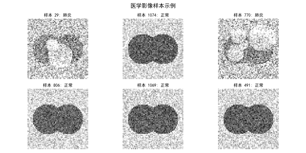
6.2神经网络训练历史
这张图片包含两个子图,左侧显示训练和验证损失曲线,右侧显示训练和验证准确率曲线。通过观察这些曲线,可以评估模型的训练效果:理想情况下训练损失应逐渐下降,验证损失也应同步下降;如果验证损失开始上升而训练损失继续下降,可能出现过拟合。准确率曲线展示了模型分类能力的提升过程,帮助分析模型是否收敛、是否存在过拟合或欠拟合问题。
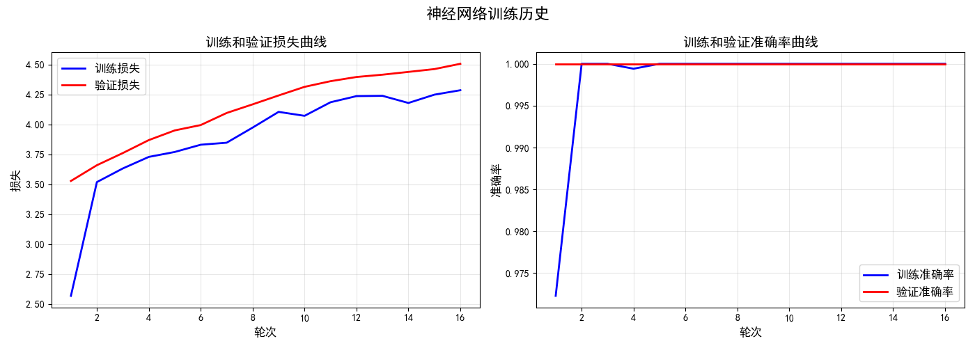
6.3测试集ROC曲线
ROC曲线展示了模型在不同分类阈值下的性能表现,横坐标为假正率(误诊率),纵坐标为真正率(检出率)。曲线越靠近左上角表示模型性能越好,曲线下的面积(AUC)量化了模型的整体判别能力。图中还包含一条从原点到右上角的对角线,代表随机猜测的性能,用于对比。ROC分析帮助确定最佳分类阈值,平衡敏感性和特异性。
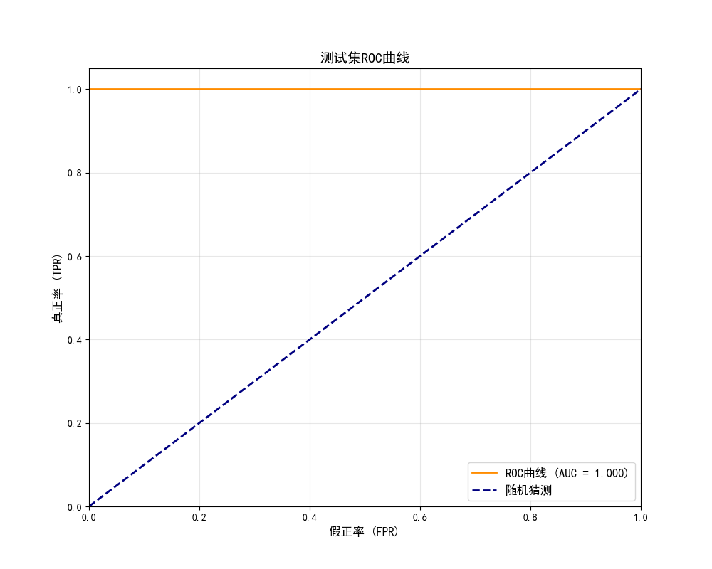
6.4测试集预测结果可视化
这张图片以网格形式展示了10个随机测试样本的预测结果。每张子图显示原始X光图像,标题包含真实诊断、预测诊断和预测概率。错误预测的样本会用红色边框突出显示,直观展示模型在具体病例上的表现。这种可视化帮助识别模型容易混淆的病例类型,理解模型决策的可信度,并发现可能的模式错误。
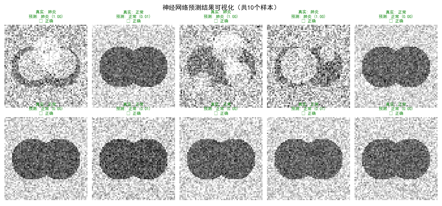
6.5测试集混淆矩阵热图
混淆矩阵热图以颜色编码的形式展示了模型分类结果的四种类别:真正例(正确识别肺炎)、真负例(正确识别正常)、假正例(误将正常诊断为肺炎)、假负例(漏诊肺炎)。热图颜色深浅表示数量多少,数值标注在格子内。通过混淆矩阵,可以清晰了解模型的错误类型分布,这对医疗诊断尤其重要,因为不同类型错误的临床意义不同。
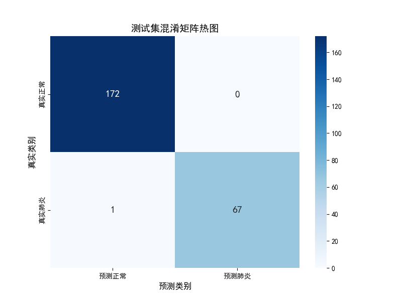
6.6单个病例诊断报告(共5张)
这五张图片分别展示了对5个随机测试病例的详细诊断报告。每张图分为左右两部分:左侧显示肺部X光影像,右侧以格式化文本展示AI诊断结果,包括预测类别、概率值、置信度评估、具体医疗建议和诊断时间戳。如果已知真实诊断,还会标注AI判断是否正确。不同诊断结果使用不同背景颜色(肺炎为浅红,正常为浅绿),增强视觉区分。


6.6诊断统计图表
最后一张图片包含两个统计子图:左侧饼图显示诊断病例中正常与肺炎的比例分布,右侧柱状图展示诊断结果的置信度分布(高、中、低置信度各占多少)。这张图表提供了批量诊断的宏观统计信息,帮助评估模型在实际应用中的整体表现和可靠性,对于临床部署和质量控制具有重要意义。
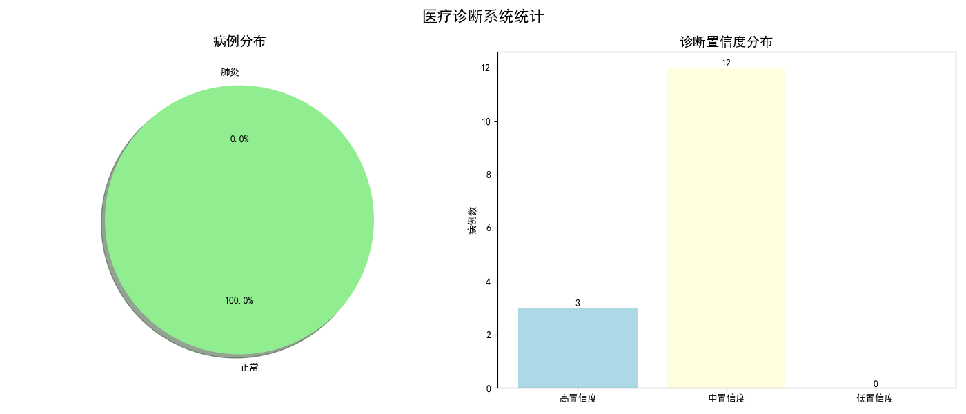
6.7diagnosis_history.csv
diagnosis_history.csv 是一个记录了医学影像辅助诊断系统所有诊断历史的数据文件,它系统性地保存了每次诊断的详细信息,包括图像ID、预测结果(正常/肺炎)、预测概率、置信度评估、具体医疗建议以及时间戳等关键数据。这个文件的主要作用是提供完整的诊断追溯和审计记录,便于医生复核AI诊断的准确性、分析模型在不同病例上的表现、监测系统运行质量,并为后续的模型优化和临床研究提供宝贵的数据支持。
|----------|------------|---------------------|------------|------------------------------------------|-----------------|
| image_id | prediction | probability | confidence | recommendation | timestamp |
| test_178 | 正常 | 0.2028839445888495 | 中置信度 | 肺部影像基本正常,建议: 1. 如有症状请咨询医生 2. 保持健康生活方式 | 2025/12/5 20:03 |
| test_128 | 正常 | 0.17355567056667487 | 中置信度 | 肺部影像未见明显异常,建议: 1. 常规健康体检 2. 如有呼吸道症状请咨询医生 | 2025/12/5 20:04 |
| test_66 | 正常 | 0.20034686221512973 | 中置信度 | 肺部影像基本正常,建议: 1. 如有症状请咨询医生 2. 保持健康生活方式 | 2025/12/5 20:04 |
| test_130 | 正常 | 0.9681952699028739 | 高置信度 | 肺部影像基本正常,建议: 1. 如有症状请咨询医生 2. 保持健康生活方式 | 2025/12/5 20:04 |
| test_110 | 正常 | 0.18668140350306728 | 中置信度 | 肺部影像未见明显异常,建议: 1. 常规健康体检 2. 如有呼吸道症状请咨询医生 | 2025/12/5 20:04 |
| 5 | 正常 | 0.15479885845837102 | 中置信度 | 肺部影像未见明显异常,建议: 1. 常规健康体检 2. 如有呼吸道症状请咨询医生 | 2025/12/5 20:04 |
| 1 | 正常 | 0.9011161456267888 | 高置信度 | 肺部影像基本正常,建议: 1. 如有症状请咨询医生 2. 保持健康生活方式 | 2025/12/5 20:04 |
| 2 | 正常 | 0.23239949449524952 | 中置信度 | 肺部影像基本正常,建议: 1. 如有症状请咨询医生 2. 保持健康生活方式 | 2025/12/5 20:04 |
| 3 | 正常 | 0.23145277760111954 | 中置信度 | 肺部影像基本正常,建议: 1. 如有症状请咨询医生 2. 保持健康生活方式 | 2025/12/5 20:04 |
| 4 | 正常 | 0.2028839445888495 | 中置信度 | 肺部影像基本正常,建议: 1. 如有症状请咨询医生 2. 保持健康生活方式 | 2025/12/5 20:04 |
| 5 | 正常 | 0.2385117338212506 | 中置信度 | 肺部影像基本正常,建议: 1. 如有症状请咨询医生 2. 保持健康生活方式 | 2025/12/5 20:04 |
| 6 | 正常 | 0.18613690772568636 | 中置信度 | 肺部影像未见明显异常,建议: 1. 常规健康体检 2. 如有呼吸道症状请咨询医生 | 2025/12/5 20:04 |
| 7 | 正常 | 0.8429319150888995 | 中置信度 | 肺部影像基本正常,建议: 1. 如有症状请咨询医生 2. 保持健康生活方式 | 2025/12/5 20:04 |
| 8 | 正常 | 0.23572734953672228 | 中置信度 | 肺部影像基本正常,建议: 1. 如有症状请咨询医生 2. 保持健康生活方式 | 2025/12/5 20:04 |
| 9 | 正常 | 0.8799000219928474 | 高置信度 | 肺部影像基本正常,建议: 1. 如有症状请咨询医生 2. 保持健康生活方式 | 2025/12/5 20:04 |