引言
感知器(Perceptron)是神经网络的基础构建块,由 Frank Rosenblatt 于 1957 年提出,是最早的监督学习算法之一。它用于解决线性可分的二分类问题,虽然结构简单,但蕴含了神经网络的核心思想 ------ 通过调整权重来学习输入与输出之间的映射关系。
一、感知器算法原理
1. 数学模型
感知器的数学模型可以表示为:
其中:
是输入特征向量
- b 是偏置项
- y 是输出
2. 激活函数
本文使用对称硬性极限激活函数:
3. 学习规则
感知器的学习规则基于错误修正:当预测结果与真实标签不符时,根据误差调整权重和偏置。更新公式为:
其中:
- y 是真实标签
二、代码实现
1. 环境准备
python
import numpy as np
import matplotlib.pyplot as plt
from sklearn.datasets import make_classification
2. 感知器类设计
python
class Perceptron:
    def __init__(self, learning_rate=0.01, max_epochs=100):
        """初始化感知器"""
        self.lr = learning_rate  # 学习率
        self.max_epochs = max_epochs  # 最大迭代次数
        self.w = None  # 权重向量
        self.b = 0     # 偏置
        self.final_w = None  # 最终权重
        self.final_b = 0     # 最终偏置
3. 核心方法实现
激活函数
python
def activate(self, z):
    """对称硬性极限激活函数"""
    return 1 if z >= 0 else -1
预测方法
python
def predict(self, x):
    """单样本预测"""
    return self.activate(np.dot(x, self.w) + self.b)
决策线绘制
python
def _plot_decision_line(self, ax, X, w, b):
    """内部辅助函数:绘制决策线"""
    x1 = np.linspace(X[:, 0].min()-1, X[:, 0].max()+1, 100)
    if abs(w[1]) > 1e-6:
        x2 = (-w[0]*x1 - b) / w[1]
    else:
        x1 = [-b/(w[0]+1e-6)]*100  # 垂直决策线
        x2 = np.linspace(X[:, 1].min()-1, X[:, 1].max()+1, 100)
    ax.plot(x1, x2, 'k-', linewidth=2)
    return ax
训练核心逻辑
python
def train(self, X, y):
"""核心训练逻辑"""
y_sym = np.where(y==0, -1, 1) # 将标签转换为-1和1
n_samples, n_features = X.shape
self.w = np.zeros(n_features) # 初始化权重为0
self.b = 0
epoch_params = [] # 保存每轮迭代的参数,用于可视化
for epoch in range(self.max_epochs):
updated = False
for i in range(n_samples):
y_pred = self.predict(X[i])
if y_pred != y_sym[i]:
# 参数更新
self.w += self.lr * (y_sym[i] - y_pred) * X[i]
self.b += self.lr * (y_sym[i] - y_pred)
updated = True
epoch_params.append((self.w.copy(), self.b.copy()))
if not updated:
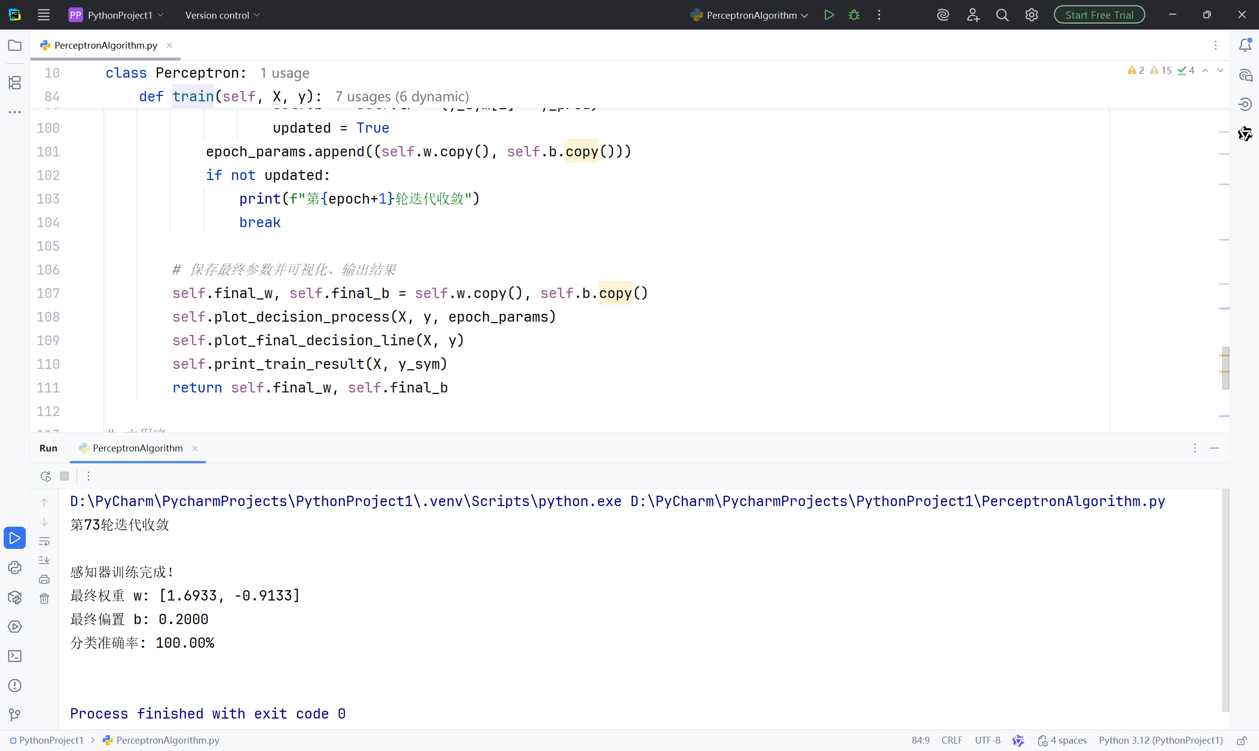
print(f"第{epoch+1}轮迭代收敛")
break
# 保存最终参数并可视化、输出结果
self.final_w, self.final_b = self.w.copy(), self.b.copy()
self.plot_decision_process(X, y, epoch_params)
self.plot_final_decision_line(X, y)
self.print_train_result(X, y_sym)
return self.final_w, self.final_b4. 可视化与结果输出
python
def plot_decision_process(self, X, y, epoch_params):
"""简化决策线过程可视化"""
total = len(epoch_params)
n_plots = min(5, total)
step = max(1, total//n_plots)
selected = epoch_params[::step][:n_plots]
for idx, (w, b) in enumerate(selected):
fig, ax = plt.subplots(figsize=(7, 3))
# 绘制样本
ax.scatter(X[y==0][:,0], X[y==0][:,1], c='red', label='类别0(-1)', edgecolors='k', s=20)
ax.scatter(X[y==1][:,0], X[y==1][:,1], c='blue', label='类别1(1)', edgecolors='k', s=20)
# 绘制决策线
self._plot_decision_line(ax, X, w, b)
# 基础配置
ax.set_xlabel('特征1'), ax.set_ylabel('特征2')
ax.set_title(f'迭代{idx*step+1}'), ax.legend(), ax.grid(alpha=0.3)
plt.savefig(f'perceptron_epoch_{idx*step+1}.png', bbox_inches='tight')
plt.close()
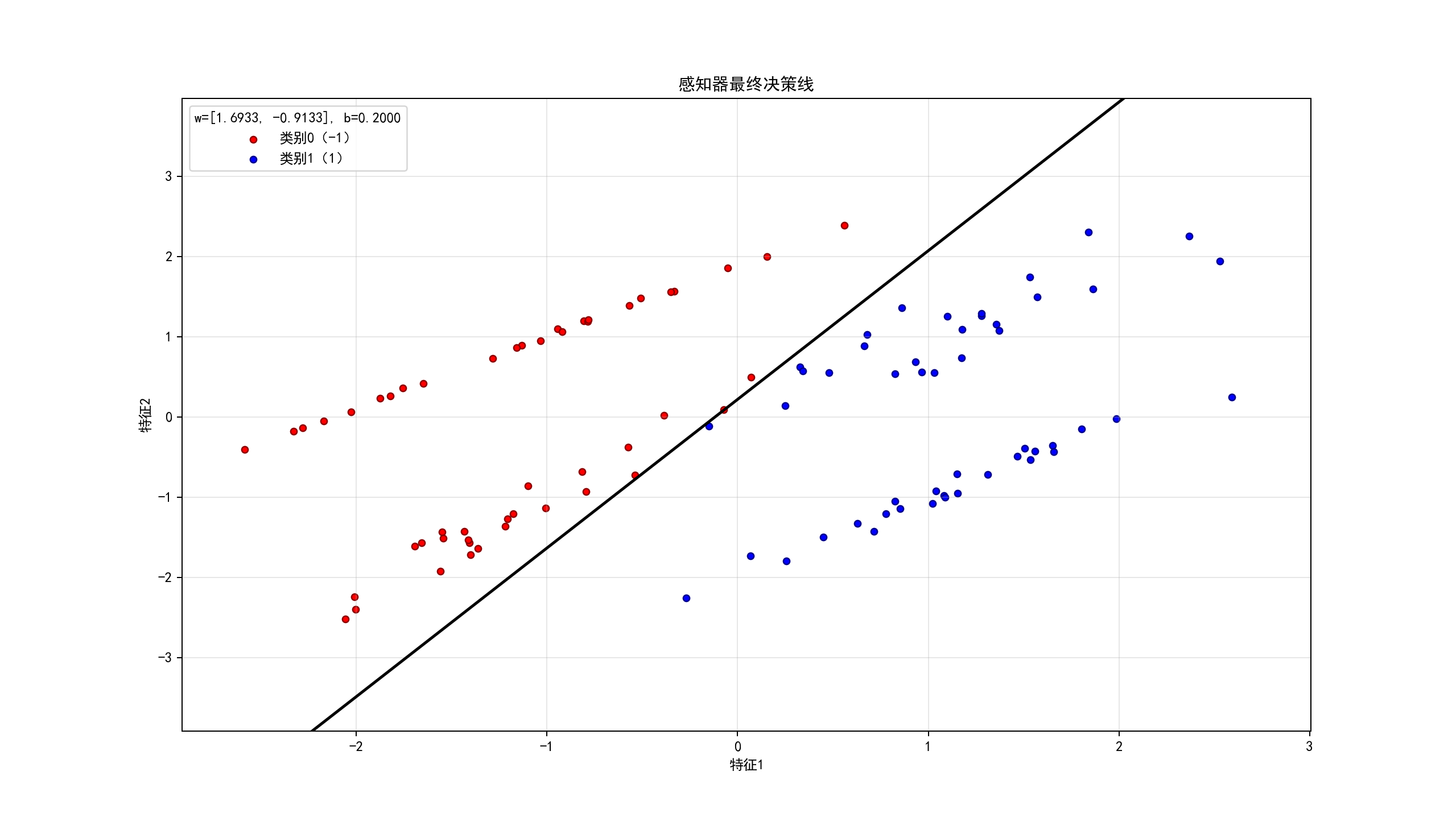
def plot_final_decision_line(self, X, y):
"""最终决策线"""
fig, ax = plt.subplots(figsize=(7, 3))
# 绘制样本
ax.scatter(X[y==0][:,0], X[y==0][:,1], c='red', label='类别0(-1)', edgecolors='darkred', s=20)
ax.scatter(X[y==1][:,0], X[y==1][:,1], c='blue', label='类别1(1)', edgecolors='darkblue', s=20)
# 绘制最终决策线
self._plot_decision_line(ax, X, self.final_w, self.final_b)
# 配置
ax.set_xlabel('特征1'), ax.set_ylabel('特征2')
ax.set_title('感知器最终决策线')
ax.legend(title=f'w=[{self.final_w[0]:.4f}, {self.final_w[1]:.4f}], b={self.final_b:.4f}')
ax.grid(alpha=0.3)
plt.savefig('感知器_最终决策线.png', dpi=150, bbox_inches='tight')
plt.show()
def print_train_result(self, X, y_sym):
"""简化训练结果输出"""
print("\n感知器训练完成!")
print(f"最终权重 w: [{self.final_w[0]:.4f}, {self.final_w[1]:.4f}]")
print(f"最终偏置 b: {self.final_b:.4f}")
# 向量化预测计算准确率
y_pred = np.apply_along_axis(self.predict, 1, X)
print(f"分类准确率: {np.mean(y_pred == y_sym):.2%}\n")三、完整代码
python
import numpy as np
import matplotlib.pyplot as plt
from sklearn.datasets import make_classification

# 全局绘图设置
plt.rcParams['font.sans-serif'] = ['SimHei']
plt.rcParams['axes.unicode_minus'] = False
plt.rcParams['figure.dpi'] = 120

class Perceptron:
    def __init__(self, learning_rate=0.01, max_epochs=100):
        """初始化感知器"""
        self.lr = learning_rate
        self.max_epochs = max_epochs
        self.w = None  # 权重 (n_features,)
        self.b = 0     # 偏置
        self.final_w = None
        self.final_b = 0

    def activate(self, z):
        """对称硬性极限激活函数"""
        return 1 if z >= 0 else -1

    def predict(self, x):
        """单样本预测"""
        return self.activate(np.dot(x, self.w) + self.b)

    def _plot_decision_line(self, ax, X, w, b):
        """内部辅助函数:绘制决策线"""
        x1 = np.linspace(X[:, 0].min()-1, X[:, 0].max()+1, 100)
        if abs(w[1]) > 1e-6:
            x2 = (-w[0]*x1 - b) / w[1]
        else:
            x1 = [-b/(w[0]+1e-6)]*100  # 垂直决策线
            x2 = np.linspace(X[:, 1].min()-1, X[:, 1].max()+1, 100)
        ax.plot(x1, x2, 'k-', linewidth=2)
        return ax

    def plot_decision_process(self, X, y, epoch_params):
        """简化决策线过程可视化"""
        total = len(epoch_params)
        n_plots = min(5, total)
        step = max(1, total//n_plots)
        selected = epoch_params[::step][:n_plots]

        for idx, (w, b) in enumerate(selected):
            fig, ax = plt.subplots(figsize=(7, 3))
            # 绘制样本
            ax.scatter(X[y==0][:,0], X[y==0][:,1], c='red', label='类别0(-1)', edgecolors='k', s=20)
            ax.scatter(X[y==1][:,0], X[y==1][:,1], c='blue', label='类别1(1)', edgecolors='k', s=20)
            # 绘制决策线
            self._plot_decision_line(ax, X, w, b)
            # 基础配置
            ax.set_xlabel('特征1'), ax.set_ylabel('特征2')
            ax.set_title(f'迭代{idx*step+1}'), ax.legend(), ax.grid(alpha=0.3)
            plt.savefig(f'perceptron_epoch_{idx*step+1}.png', bbox_inches='tight')
            plt.close()

    def plot_final_decision_line(self, X, y):
        """最终决策线"""
        fig, ax = plt.subplots(figsize=(7, 3))
        # 绘制样本
        ax.scatter(X[y==0][:,0], X[y==0][:,1], c='red', label='类别0(-1)', edgecolors='darkred', s=20)
        ax.scatter(X[y==1][:,0], X[y==1][:,1], c='blue', label='类别1(1)', edgecolors='darkblue', s=20)
        # 绘制最终决策线
        self._plot_decision_line(ax, X, self.final_w, self.final_b)
        # 配置
        ax.set_xlabel('特征1'), ax.set_ylabel('特征2')
        ax.set_title('感知器最终决策线')
        ax.legend(title=f'w=[{self.final_w[0]:.4f}, {self.final_w[1]:.4f}], b={self.final_b:.4f}')
        ax.grid(alpha=0.3)
        plt.savefig('感知器_最终决策线.png', dpi=150, bbox_inches='tight')
        plt.show()

    def print_train_result(self, X, y_sym):
        """简化训练结果输出"""
        print("\n感知器训练完成!")
        print(f"最终权重 w: [{self.final_w[0]:.4f}, {self.final_w[1]:.4f}]")
        print(f"最终偏置 b: {self.final_b:.4f}")
        # 向量化预测计算准确率
        y_pred = np.apply_along_axis(self.predict, 1, X)
        print(f"分类准确率: {np.mean(y_pred == y_sym):.2%}\n")

    def train(self, X, y):
        """核心训练逻辑"""
        y_sym = np.where(y==0, -1, 1)  # 标签转换
        n_samples, n_features = X.shape
        self.w = np.zeros(n_features)
        self.b = 0
        epoch_params = []

        for epoch in range(self.max_epochs):
            updated = False
            for i in range(n_samples):
                y_pred = self.predict(X[i])
                if y_pred != y_sym[i]:
                    # 参数更新
                    self.w += self.lr * (y_sym[i] - y_pred) * X[i]
                    self.b += self.lr * (y_sym[i] - y_pred)
                    updated = True
            epoch_params.append((self.w.copy(), self.b.copy()))
            if not updated:
                print(f"第{epoch+1}轮迭代收敛")
                break

        # 保存最终参数并可视化、输出结果
        self.final_w, self.final_b = self.w.copy(), self.b.copy()
        self.plot_decision_process(X, y, epoch_params)
        self.plot_final_decision_line(X, y)
        self.print_train_result(X, y_sym)
        return self.final_w, self.final_b

# 主程序
if __name__ == "__main__":
    # 生成线性可分二分类数据
    X, y = make_classification(
        n_samples=100, n_features=2, n_informative=2, n_redundant=0,
        n_classes=2, random_state=42
    )

    # 训练感知器
    perceptron = Perceptron(learning_rate=0.1, max_epochs=100)
    perceptron.train(X, y)
四、实验结果