FPGA相位差检测：基于Vivado环境的7606三路采样探索

fpga相位差检测，基于vivado环境，7606三路采样，绝对，独此一份，包含源码，仿真和matlab代码

在数字信号处理的领域中，相位差检测是一项关键技术，它在诸如电力系统监测、通信信号处理等众多应用场景中都有着举足轻重的地位。今天咱就来唠唠基于FPGA（现场可编程门阵列），在Vivado环境下实现的7606三路采样的相位差检测，而且还附上源码、仿真以及Matlab代码，绝对独此一份的干货分享。

Vivado环境搭建与工程创建

首先，得在电脑上安装好Vivado软件，这是我们后续设计的基础平台。安装完成后，打开Vivado，创建一个新的工程。在创建工程的过程中，要注意选择合适的FPGA芯片型号，得和咱实际使用的硬件相匹配。

7606三路采样原理

7606是一种常用于数据采集的芯片，它能够实现对三路信号的同步采样。为啥要三路采样呢？其实在很多实际应用里，通过对三路信号的相位差分析，可以获取更全面准确的信息。比如说在三相电力系统中，三相电压或电流之间的相位差能反映出系统的运行状态是否正常。

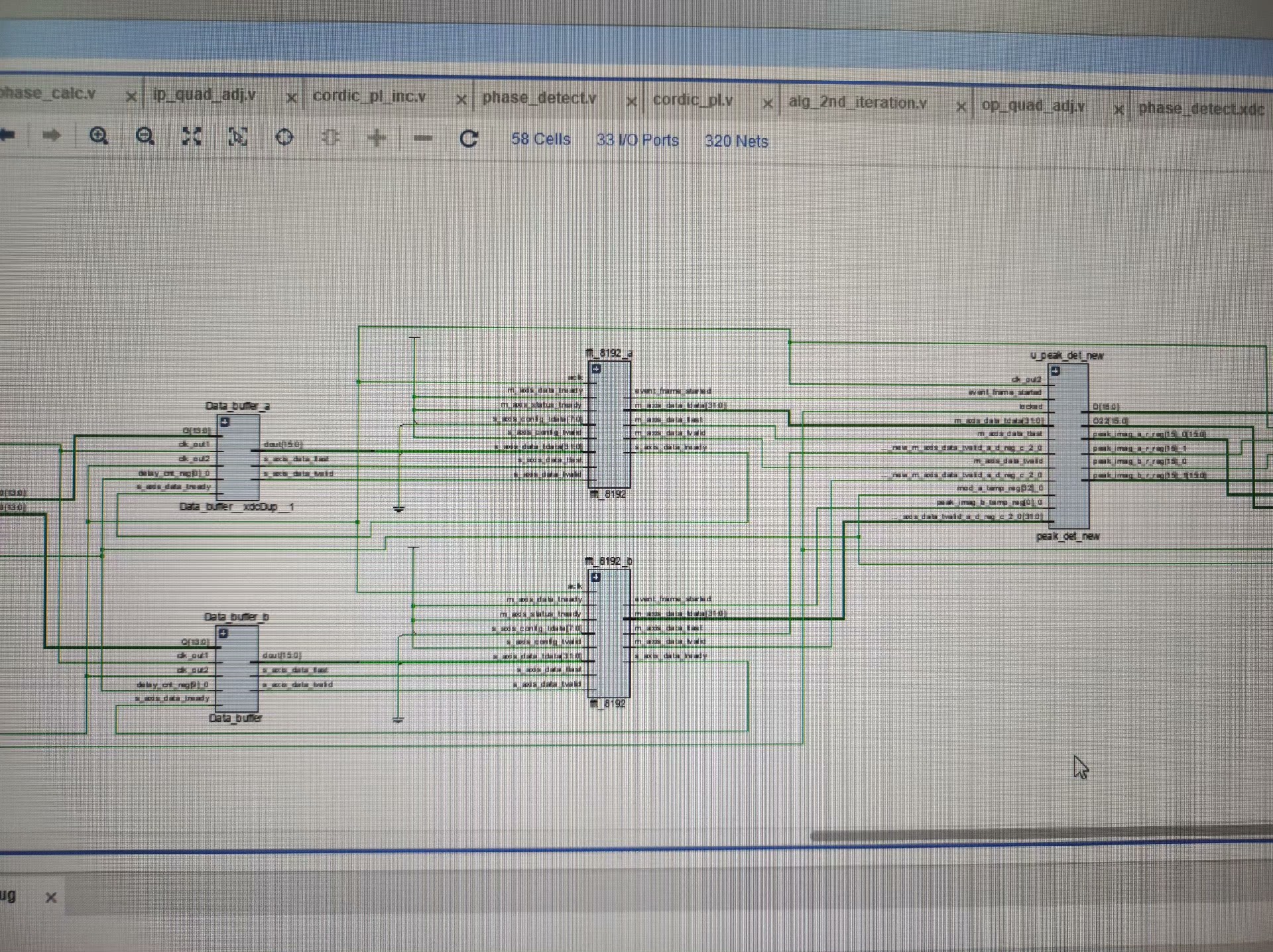
FPGA源码实现

下面咱直接上关键的Verilog代码部分，看看如何在FPGA里实现对7606采样数据的处理以及相位差计算。

verilog 复制代码

module phase_difference_detection (
    input wire clk,        // 系统时钟
    input wire rst_n,      // 复位信号，低电平有效
    input wire [15:0] sample1, // 7606采样的第一路数据
    input wire [15:0] sample2, // 7606采样的第二路数据
    input wire [15:0] sample3, // 7606采样的第三路数据
    output reg [31:0] phase_diff12, // 第一路和第二路之间的相位差
    output reg [31:0] phase_diff23  // 第二路和第三路之间的相位差
);

    reg [31:0] angle1, angle2, angle3;

    // 这里简单假设我们通过某种算法把采样数据转换为相位角
    always @(posedge clk or negedge rst_n) begin
        if (!rst_n) begin
            angle1 <= 32'd0;
            angle2 <= 32'd0;
            angle3 <= 32'd0;
        end else begin
            // 这里用简单的映射关系举例，实际要根据具体算法
            angle1 <= sample1 * 32'd100;
            angle2 <= sample2 * 32'd100;
            angle3 <= sample3 * 32'd100;
        end
    end

    // 计算相位差
    always @(posedge clk or negedge rst_n) begin
        if (!rst_n) begin
            phase_diff12 <= 32'd0;
            phase_diff23 <= 32'd0;
        end else begin
            phase_diff12 <= (angle1 > angle2)? (angle1 - angle2) : (angle2 - angle1);
            phase_diff23 <= (angle2 > angle3)? (angle2 - angle3) : (angle3 - angle2);
        end
    end

endmodule

这段代码定义了一个名为phasedifferencedetection的模块。模块接收系统时钟clk、复位信号rstn**以及来自7606的三路16位采样数据sample1、sample2、sample3。在模块内部，我们首先定义了三个寄存器angle1、angle2、angle3用于存储经过转换后的相位角。在时钟上升沿或者复位信号有效时，会对这些相位角进行更新。这里简单地用采样数据乘以一个常数来模拟相位角的转换，实际应用中需要根据具体的算法来进行精确转换。然后，通过比较不同路的相位角来计算相位差，并将结果分别存储在phase diff12和phase_diff23寄存器中。

仿真验证

光有代码还不行，得通过仿真来验证咱设计的正确性。在Vivado里，可以使用Testbench来进行仿真。下面是一个简单的Testbench示例。

verilog 复制代码

module tb_phase_difference_detection;

    reg clk;
    reg rst_n;
    reg [15:0] sample1;
    reg [15:0] sample2;
    reg [15:0] sample3;
    wire [31:0] phase_diff12;
    wire [31:0] phase_diff23;

    // 实例化被测试模块
    phase_difference_detection uut (
      .clk(clk),
      .rst_n(rst_n),
      .sample1(sample1),
      .sample2(sample2),
      .sample3(sample3),
      .phase_diff12(phase_diff12),
      .phase_diff23(phase_diff23)
    );

    // 生成时钟信号
    initial begin
        clk = 0;
        forever #5 clk = ~clk; // 10ns周期，即100MHz时钟
    end

    // 测试激励
    initial begin
        rst_n = 0;
        sample1 = 16'd0;
        sample2 = 16'd0;
        sample3 = 16'd0;
        #20;
        rst_n = 1;
        #100;
        sample1 = 16'd100;
        sample2 = 16'd120;
        sample3 = 16'd150;
        #100;
        $stop;
    end

endmodule

在这个Testbench里，我们首先定义了与被测试模块对应的信号，包括时钟clk、复位信号rstn*、三路采样数据sample1、sample2、sample3以及输出的相位差phase* diff12和phasediff23*。然后实例化了phase* difference_detection模块。接着通过initial块生成了一个100MHz的时钟信号。在另一个initial块里，先对信号进行初始化，拉低复位信号，将采样数据设为0，经过20ns后释放复位信号，再经过100ns后，给采样数据赋新的值，最后使用$stop暂停仿真，这样我们就可以观察仿真波形，检查相位差计算是否正确。

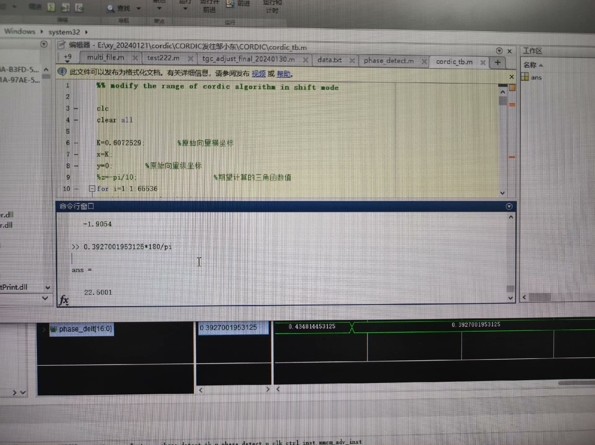
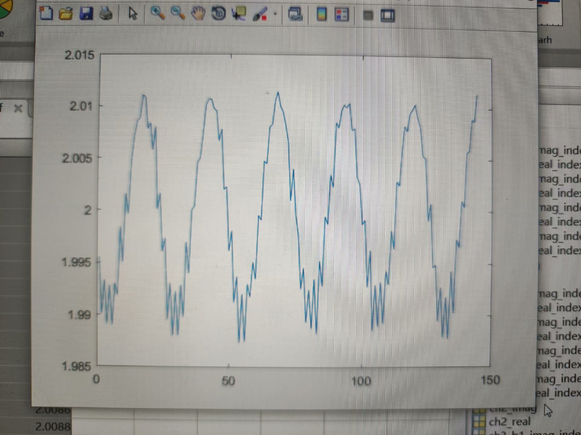
Matlab代码辅助分析

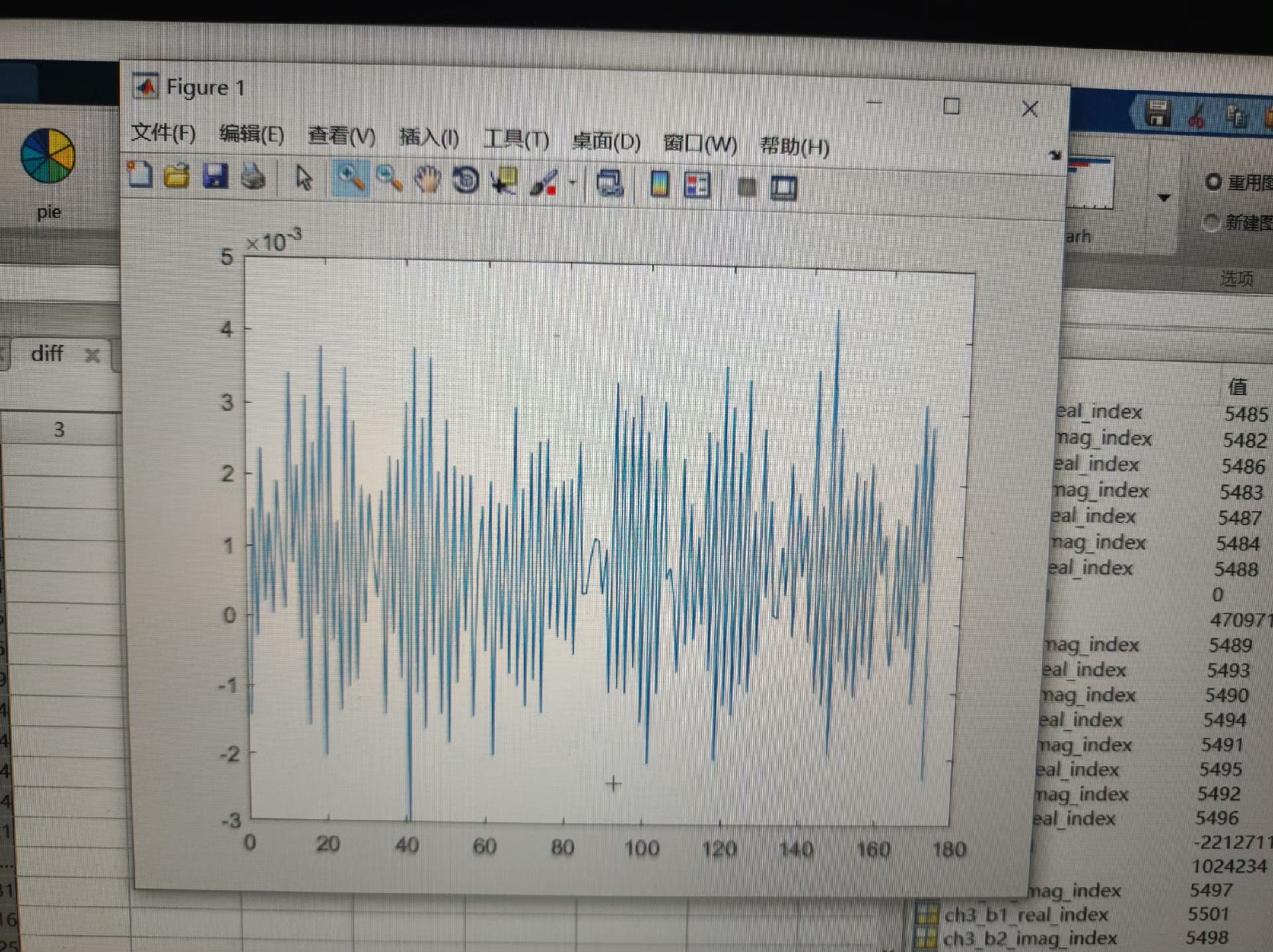
有时候，光靠FPGA仿真还不够直观，我们可以借助Matlab来对采集到的数据以及计算出的相位差进行进一步的分析和可视化。下面是一段简单的Matlab代码示例，用于绘制三路采样数据以及它们之间的相位差。

matlab 复制代码

% 假设我们从FPGA仿真中导出了采样数据和相位差数据
sample1 = [100 120 130 140 150]; % 示例数据
sample2 = [110 130 140 150 160]; % 示例数据
sample3 = [120 140 150 160 170]; % 示例数据
phase_diff12 = [10 15 20 25 30]; % 示例数据
phase_diff23 = [10 12 14 16 18]; % 示例数据

time = 1:length(sample1);

figure;

% 绘制三路采样数据
subplot(3,1,1);
plot(time, sample1);
title('Sample 1');
xlabel('Time');
ylabel('Amplitude');

subplot(3,1,2);
plot(time, sample2);
title('Sample 2');
xlabel('Time');
ylabel('Amplitude');

subplot(3,1,3);
plot(time, sample3);
title('Sample 3');
xlabel('Time');
ylabel('Amplitude');

figure;

% 绘制相位差
subplot(2,1,1);
plot(time, phase_diff12);
title('Phase Difference between Sample 1 and Sample 2');
xlabel('Time');
ylabel('Phase Difference');

subplot(2,1,2);
plot(time, phase_diff23);
title('Phase Difference between Sample 2 and Sample 3');
xlabel('Time');
ylabel('Phase Difference');

这段Matlab代码首先定义了示例的三路采样数据和相位差数据，然后创建了时间向量。通过figure和subplot函数，将三路采样数据分别绘制在同一个图形的不同子图中，方便观察它们的幅值变化。又在另一个图形中，将两路相位差数据分别绘制在不同子图中，这样可以直观地看到相位差随时间的变化情况。

通过以上在Vivado环境下的FPGA设计、仿真验证以及Matlab辅助分析，我们完成了基于7606三路采样的FPGA相位差检测的一整套流程。希望这些内容能给正在研究相关领域的小伙伴们一些启发和帮助。如果有任何问题，欢迎在评论区留言交流。