原文链接
自己看的机翻和kimi和一些笔记
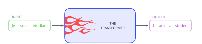
A High-Level Look
把模型看成黑箱,输入是一种语言,输出翻译成另一种语言
编码器有六层、解码器六层
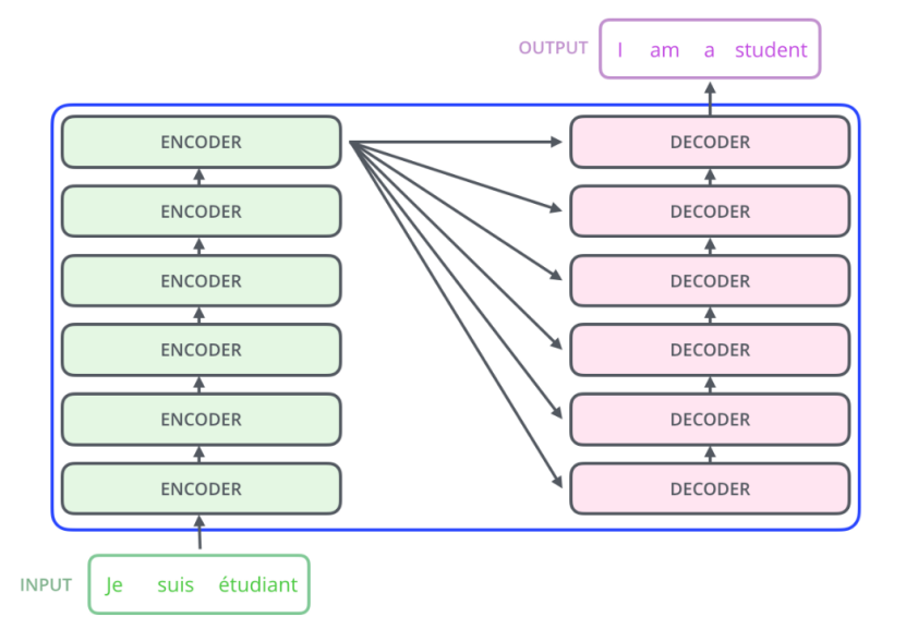
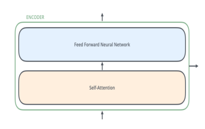
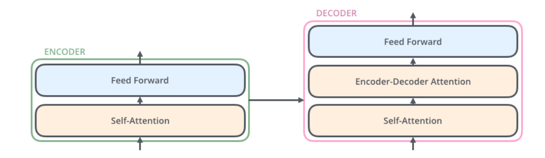
编码器self-attention+ffn,解码器多了一层self-attention,帮助解码器关注相关的输入序列
Bringing The Tensors Into The Picture
现在我们已经看到了模型的主要组件,让我们开始查看各种向量/张量,以及它们如何在这些组件之间流动,从而将经过训练的模型的输入转化为输出。
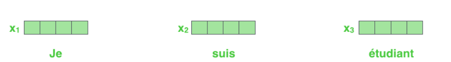
与一般的NLP应用程序一样,我们首先使用嵌入算法将每个输入单词转换为向量。(每个单词被嵌入到大小为512的向量中。我们将用这些简单的方框来表示这些向量。)
嵌入只发生在最底层的编码器中bottom-most encoder。对于所有编码器来说,共同的抽象是它们接收一个向量列表,每个向量的大小为512。在底部的编码器中输入是单词Embedding,但在其他编码器中,输入是前一个的编码器(the encoder that's directly below)的输出。
这个列表的大小是我们可以设置的超参数-基本上是我们训练数据集中最长句子的长度。
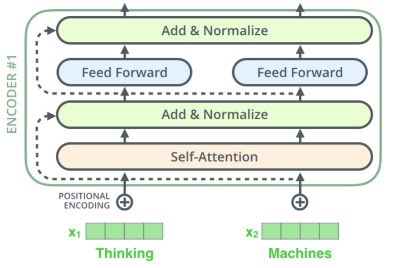
在我们的输入序列中嵌入单词之后,每个单词都流经编码器的两层。
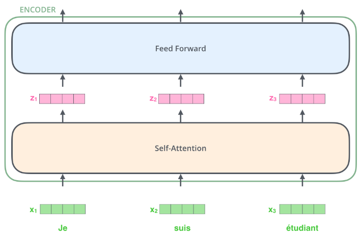
在这里,我们开始看到Transformer的一个关键属性,即每个位置的单词在编码器中流经其自己的路径the word in each position flows through its own path in the encoder。在自我关注层,这些路径之间存在依赖关系。然而,前馈层不具有这些依赖性,因此各种路径可以在流经前馈层时并行执行。
Now We're Encoding!
Self-Attention at a High Level
The animal didn't cross the street because it was too tired
要知道it的含义
这句
话中的it指的是什么?它指的是街道还是动物?这对人类来说是一个简单的问题,但对算法来说就不那么简单了。当模型处理单词"it"时,自我注意使其将"it"与"动物"联系起来。
当模型处理每个单词(输入序列中的每个位置)时,自我注意允许它查看输入序列中的其他位置,以寻找有助于对该单词进行更好编码的线索。As the model processes each word (each position in the input sequence), self attention allows it to look at other positions in the input sequence for clues that can help lead to a better encoding for this word.
即除了查看要处理的这个单词,还要查看其他的单词来帮助编码
RNN 通过维护一个隐藏状态(hidden state),能够将之前处理过的词语或向量的信息,与当前正在处理的词语或向量结合起来。maintain a hidden state allows an RNN to incorporate its representation of previous words/vectors it has processed with the current one it's processing.自我关注是Transformer用来把对其他相关单词的"理解"变成我们目前正在处理的单词的方法。
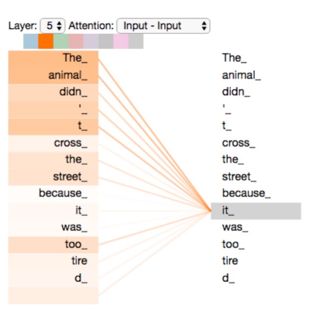
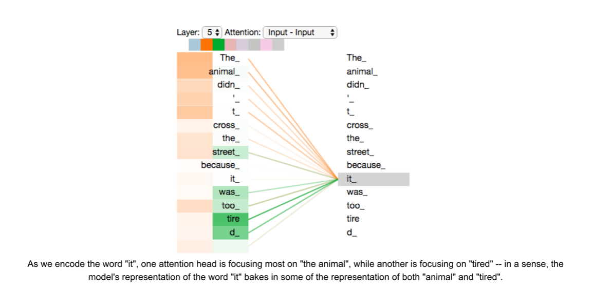
当我们在编码器#5(堆栈中最顶端的编码器)中对单词"it"进行编码时,注意力机制的一部分集中在"the Animal"上,并将其表示的一部分加入到"it"的编码中。
Self-Attention in Detail
first step:
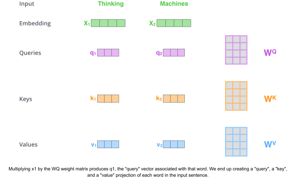
create three vectors from each of the encoder's input vectors每个输入向量都创造三个向量Q,K,V
create a Query vector, a Key vector, and a Value vector.
它们不一定要更小,这是一种架构选择,可以使多头注意力的计算(主要)保持恒定。
new vectors are smaller in dimension than the embedding vector
Q,K,V比输入的嵌入向量维度更小
Their dimensionality is 64, while the embedding and encoder input/output vectors have dimensionality of 512
它们的维度为64,而嵌入和编码器输入/输出向量的维度为512
second step:
calculate a score
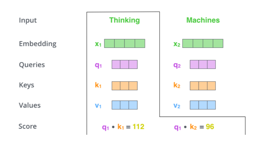
假设我们计算的是本例中第一个单词"思考"的自我注意力。我们需要对输入句子中的每个单词与该单词进行评分。分数决定了当我们在某个位置编码一个单词时,在输入句子的其他部分上的关注度。how much focus to place
分数的计算方法是将查询向量与我们要评分的单词的关键字向量相乘
the dot product of the query vector with the key vector
因此,如果我们处理的是位置为1的单词的自我注意,第一个分数将是Q1和K1的点积。第二个分数是Q1和K2的点积。
third and fourth steps
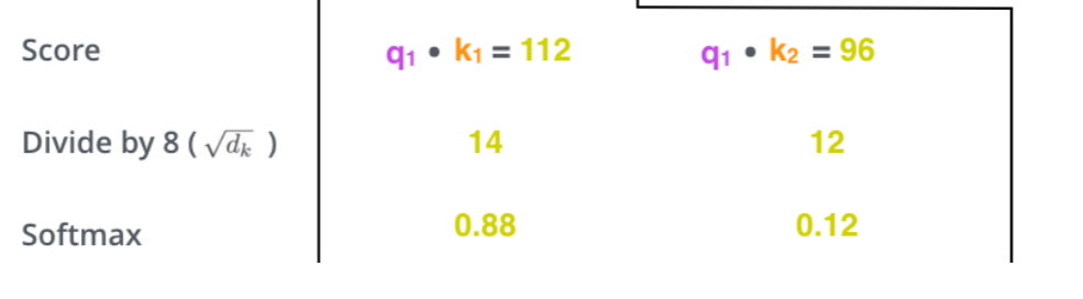
(1)divide the scores by 8将分数除以8
论文中:the square root of the dimension of the key vectors used in the paper -- 64.
即,
这会导致具有更稳定的渐变。这里可能还有其他可能的值,但这是默认设置
(2)softmax
Softmax将分数归一化normalizes,使它们都是正数并相加为1。
112/8=14
96/8=12
u=(14+12)/2=13
=(1+1)/2=
fifth step
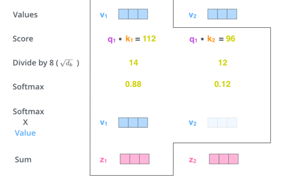
multiply each value vector by the softmax score
将每个值向量乘以Softmax分数(为给他们加起来做准备)
The intuition here is to keep intact the values of the word(s) we want to focus on, and drown-out irrelevant words (by multiplying them by tiny numbers like 0.001, for example).
这里的直觉是保持我们想要关注的单词的价值不变,并淹没不相关的单词(例如,通过将它们乘以0.001这样的微小数字)。
sixth step
sum up the weighted value vectors
把向量加起来
This produces the output of the self-attention layer at this position (for the first word)
这会在这个位置产生自我关注层的输出(对于第一个单词)
Matrix Calculation of Self-Attention
first step
calculate the Query, Key, and Value matrices
计算Q,K,V的矩阵
packing our embeddings into a matrix X, and multiplying it by the weight matrices we've trained (WQ, WK, WV).
将我们的嵌入打包到一个矩阵X中,并将其乘以我们训练过的权重矩阵(WQ,WK,WV)。
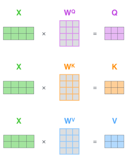
X矩阵中的每一行对应于输入句子中的一个单词。我们再次看到嵌入向量(512,或图中的4个boxes)和q/k/v向量(,或图中的3个boxes)的大小差异
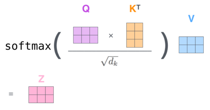
finally
因为我们处理的是矩阵,所以我们可以将第二步到第六步浓缩到一个公式中,以计算自我关注层的输出。
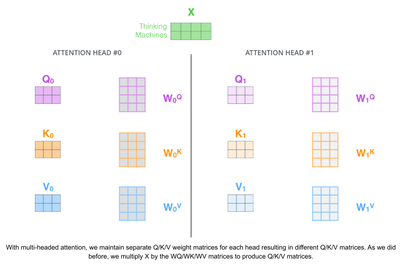
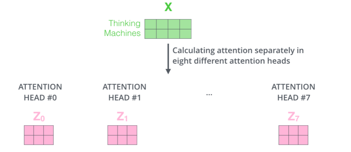
The Beast With Many Heads多头注意力
论文进一步细化了自我注意层,增加了一种称为多头注意的机制。这从两个方面改善了关注层的性能:
(1)它扩展了模型的能力,使其能够专注于不同的位置expands the model's ability to focus on different positions。是的,在上面的例子中,Z1包含了一些其他的编码,但它可能被实际的单词本身所觉得。如果我们要翻译一句话,比如""The animal didn't cross the street because it was too tired",那么知道"it"指的是哪个词将是很有用的。
(2)It gives the attention layer multiple "representation subspaces ".它为关注层提供了多个"表征子空间"。不同的注意力会产生不同的QKV,也会产生不同的Z
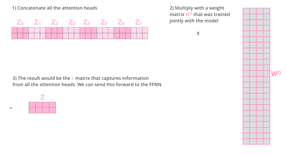
但是FFN层输入只需要一个矩阵,怎么做?
We concat the matrices then multiply them by an additional weights matrix WO.
我们拼接这些矩阵,然后将它们乘以一个附加权重矩阵。
的维度(2,24),
的维度(24,4),Z的维度(2,4)
所有矩阵概览
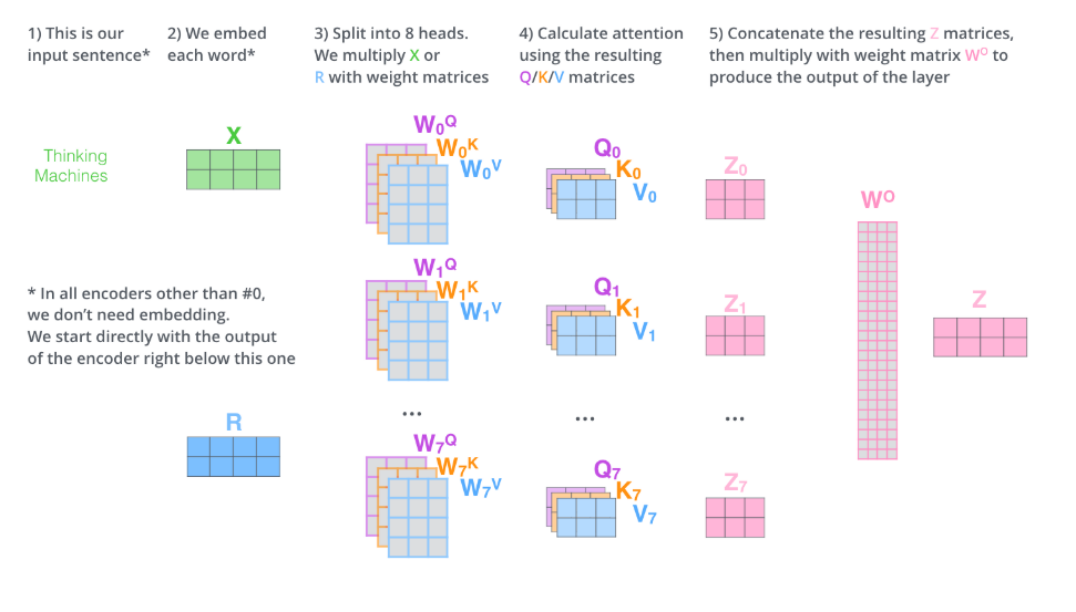
其中Z=softmax
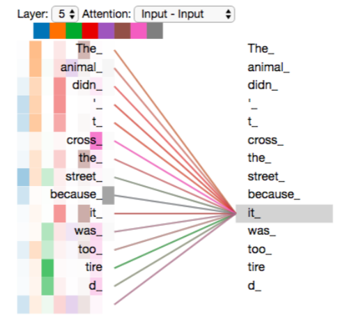
回到之前关于it应该注意"The animal didn't cross the street because it was too tired."的哪些部分,可以看到第一列animal(it指代的对象)颜色较深,第二列tire(it的状态)颜色较深
如果再加几个头就不好解释
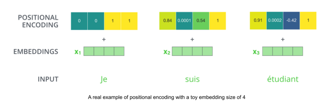
Representing The Order of The Sequence Using Positional Encoding位置编码
我们到目前为止所描述的模型中缺少的一件事是说明单词在输入序列中的顺序的方法。
为了解决这个问题,转换器向每个输入嵌入添加一个向量。这些向量遵循模型学习的特定模式,这有助于它确定每个单词的位置,或序列中不同单词之间的距离。
为什么"加"而不是"拼"?
直观理解,将这些值添加到嵌入中,在嵌入向量被投影到Q/K/V向量时,在点积注意期间,嵌入向量之间提供了有意义的距离。点积注意力计算出的相似度既反映语义也反映位置。
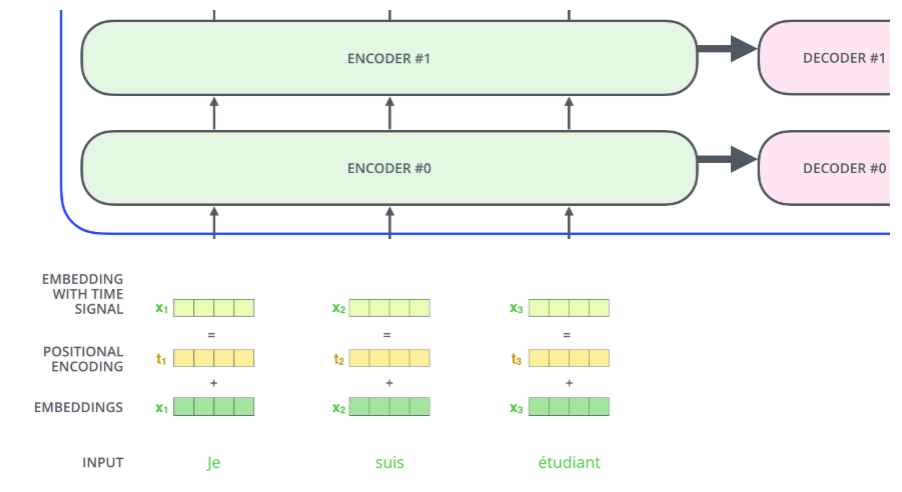
在下图中,每行对应于一个向量的位置编码。因此,第一行将是我们要添加到输入序列中第一个单词嵌入的向量。每行包含512个值-每个值都在1到-1之间。我们已经对它们进行了颜色编码,所以图案是可见的。
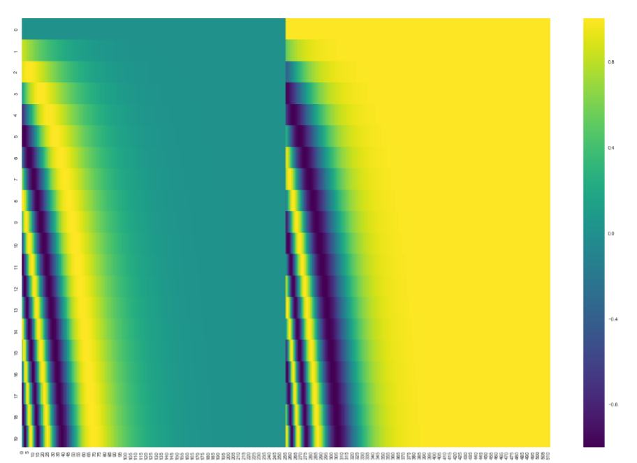
你可以看到它似乎沿着中心一分为二。这是因为左半部分的值是使用sin生成的,而右半部分是由使用cos生成的。然后将它们连接起来,形成每个位置编码向量。
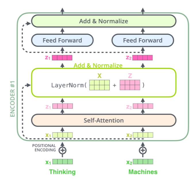
The Residuals残差连接
其实就是将输入和输出相加
解码器也有这个结构
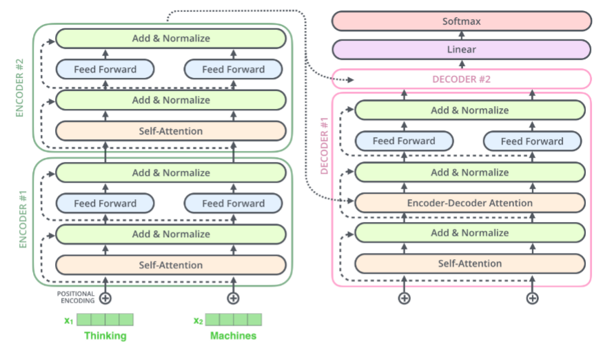
The Decoder Side解码端
The encoder starts by processing the input sequence.
先把整句输入送进左边那一摞 Encoder(通常 6 层),让它们逐层提炼特征。
The output of the top encoder is then transformed into a set of attention vectors K and V.
最顶层 Encoder 吐出的序列向量,会被复制两份,分别叫做 K(Key)和 V(Value)。
These are to be used by each decoder in its "encoder-decoder attention" layer...
每一层 Decoder 里有一个专门的子层,叫 encoder-decoder attention(也叫 cross-attention)。
这个子层让 Decoder 在生成当前词时,去左边整个输入序列里"挑重点"。
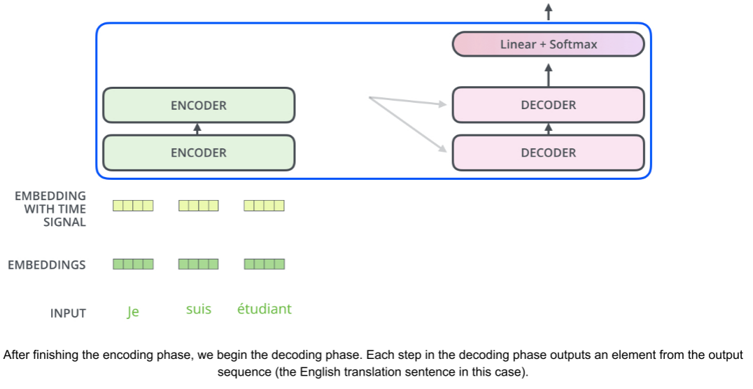
The following steps repeat the process until a special symbol is reached indicating the transformer decoder has completed its output.
不断重复"上一步输出 → 下一步输入"的循环,直到某一步蹦出 <end>(或 )这样的结束符,整个句子就算生成完了。
The output of each step is fed to the bottom decoder in the next time step.
每一步产生的词,先变成 Embedding + 位置编码,然后送进最底层 Decoder 作为新的输入。
and the decoders bubble up their decoding results just like the encoders did.
信息在 Decoder 内部也是从底层往顶层一层层传,跟 Encoder 一样;顶层 Decoder 的隐藏状态才拿去预测下一个词。
And just like we did with the encoder inputs, we embed and add positional encoding to those decoder inputs to indicate the position of each word.
别忘了给 Decoder 的输入也加上位置编码,否则模型分不清 "I love you" 和 "you love I" 的区别。
编码器和解码器的区别
1.In the decoder, the self-attention layer is only allowed to attend to earlier positions in the output sequence.
This is done by masking future positions (setting them to -inf) before the softmax step in the self-attention calculation.
解码器只能看到前面的位置,这是通过掩码实现的
2.The "Encoder-Decoder Attention" layer works just like multiheaded self-attention, except it creates itsQueries matrix from the layer below it, and takes the Keys and Values matrix from the output of the encoder stack.
编码器的Q,K,V都是来自前一层,但是解码器中的Encoder-Decoder Attention只有Q是来自前一层,K和V都是来自编码器
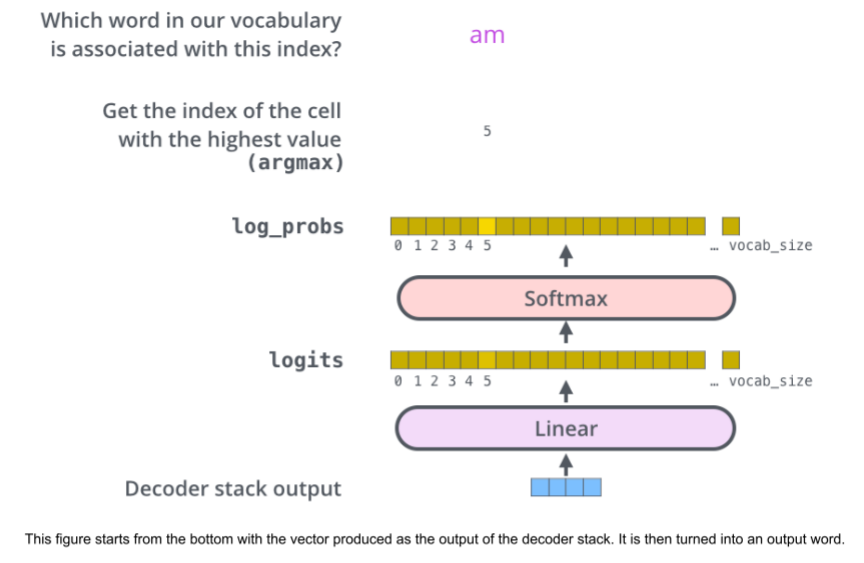
The Final Linear and Softmax Layer
解码器堆栈输出浮点向量a vector of floats。我们怎么把它变成一个词呢?这是最终的线性层的工作,紧接着是Softmax层。
1.线性层
让我们假设我们的模型知道10,000个唯一的英语单词(我们的模型的"输出词汇"),它是从它的训练数据集中学习的。这将使Logits向量有10,000个单元格宽--每个单元格对应一个唯一单词的分数。这就是我们如何解释模型的输出,然后是线性层。
The Linear layer is a simple fully connected neural network that projects the vector produced by the stack of decoders, into a much, much larger vector called a logits vector.
Linear 层做的事就是"升维":
-
假设词典有 10 000 个词,就把 512 维 → 10 000 维;
-
这 10 000 个数还没归一化,叫 logits(可以看成"原始得分")。
Let's assume that our model knows 10,000 unique English words- each cell corresponding to the score of a unique word.
-
词典大小 = 10 000;
-
于是 logits 向量长度也是 10 000;
-
第 i 个数值越大,表示模型越倾向于选第 i 个词。
我们就这样解释线性层的输出
2.Softmax
Softmax层然后将这些分数转换为概率(全部为正,全部相加为1.0)turns those scores into probabilities。选择概率最高的单元格,并生成与其相关联的单词作为该时间步长的输出。
Recap Of Training训练概述
During training, an untrained model would go through the exact same forward pass.
训练时,未经训练的模型照样走一遍 完全一样的前向计算(forward padd)
But since we are training it on a labeled training dataset, we can compare its output with the actual correct output.
因为我们有 标准答案(人工翻译的句子),可以把模型给出的概率分布与正确答案对比,算出损失(loss),然后反向传播更新权重。
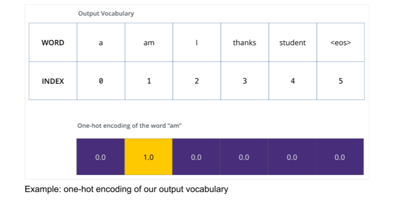
To visualize this, let's assume our output vocabulary only contains six words.
翻译:为了方便看图,我们把词典缩小到只有 6 个词:"a", "am", "I", "thanks", "student", "<eos>"(<eos> 是句子结束符)
The output vocabulary of our model is created in the preprocessing phase before we even begin training.
这份 "输出词典" 是在训练前就建好的,通常是 训练集里出现频率最高的 10 000 或 30 000 个词。
Once we define our output vocabulary, we can use a vector of the same width to indicate each word.This is also known as one-hot encoding.
一旦我们定义输出词典,我们可以使用同一宽度的向量表示单词,这也叫做one-hot encoding
So for example, we can indicate the word "am" using the following vector.
The Loss Function损失函数
由于模型的参数(权重)都是随机初始化的,因此(未训练的)模型为每个单元格/单词产生随机的概率分布。我们可以将其与实际输出进行比较,然后使用反向传播backpropagation调整tweak模型的所有权重,使输出更接近期望的输出desired output。
How do you compare two probability distributions? We simply subtract one from the other.
"比较两个概率分布"最直观就是把对应位置的概率相减(越小越接近)。
For more details, look at cross-entropy ... and Kullback--Leibler divergence ...
详细可以查 cross-entropy 和 KL divergence(交叉熵 或KL 散度)。
1.贪心解码(greedy decoding)
- Each probability distribution is represented by a vector of width vocab_size 每步输出的"概率分布"就是一条 vocab_size 维的向量。(例子中是6,实际3万或5万)
- The first probability distribution has the highest probability at the cell associated with the word "i" 第 1 步我们想让 "i" 对应的那一格概率最大(其余 29 999 格越小越好)。
- The second probability distribution has the highest probability at the cell associated with the word "am" 第 2 步想让 "am" 那一格概率最大。
- And so on, until the fifth output distribution indicates '<end of sentence> 依此类推,第 5 步想让 <eos>(结束符)那一格概率最大。
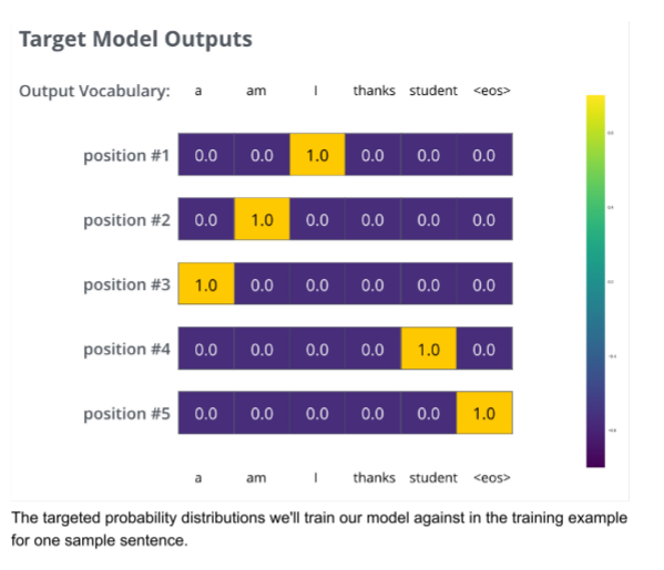
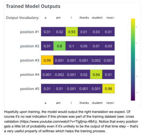
在足够大的数据集上对模型进行足够长的时间训练后,我们希望生成的概率分布如下:
2.束搜索(beam search)
Now, because the model produces the outputs one at a time,
由于模型每次只能生成一个词,必须一步一步来。
we can assume that the model is selecting the word with the highest probability from that probability distribution and throwing away the rest.
最简单的方法是------每一步都只挑概率最大的那个词,其余全扔掉。
That's one way to do it (called greedy decoding).
给这种做法起个名字:贪心解码 。
Another way to do it would be to hold on to, say, the top two words (say, 'I' and 'a' for example)
保留概率最高的前 2 个词(例如 "I" 和 "a"),而不是只留 1 个。
then in the next step, run the model twice:
下一步把模型跑两遍:
第一遍假设上一步选的是 "I";
第二遍假设上一步选的是 "a"。
once assuming the first output position was the word 'I', and another time assuming the first output position was the word 'a',
翻译:同一句话两个版本同时往下展开,各算各的概率。
and whichever version produced less error considering both positions #1 and #2 is kept.
翻译:比较这两个"半成品",看哪条路径(两个词合在一起)总体概率更高,就留哪条。
We repeat this for positions #2 and #3... etc.
翻译:继续往后走,每一步都保留当前最好的 2 条路径,再分叉、再比较、再保留......